Math 153 diary, fall 2009: second section
Later material
Previous material
In reverse order: the most recent material is first.
| Tuesday, November
10 | (Lecture
#20) |
|---|
L'Hôp
L'Hôpital's (also L'Hopital's
or L'Hospital's) Rule is a method
of evaluating certain very special limits. It is worth showing to you
because it is another neat application of "local linearization", and
some really important limits become easy to evaluate. However, it must
be used with some care. One quote I found on the Internet declared,
"Giving l'Hopital's Rule to a calculus student is like handing a
chainsaw to a three year old."
Mr. Nakamura discussed a version of L'H with you:
L'Hôpital's Rule (version 1, for 0/0)
Suppose that f and g have continuous derivatives, and that
f(a)=g(a)=0 (the eligibility criterion). If
limx→af´(x)/g´(x) exists, then
limx→af(x)/g(x) exists and is the same value.
Comment 1 It is very important to check the eligibility
criteria. For example, if you try to compute
limx→2x2/(5x+7) by instead computing
limx→22x/5 you will report the false answer 4/5
instead of the correct answer 4/17.
Comment 2 L'H is so appealing maybe because it looks like what
we all believe the Quotient Rule should be. It is a version of
paradise, maybe. (More theology is below, so please just wait.)
That's why people want to use it, even when they shouldn't.
The L'H above is called the 0/0 ("zero over zero") form. There are
other forms. For example, one version is very useful in certain
practical applications.
L'Hôpital's Rule (version 2, for ∞/∞)
Suppose that f and g have continuous derivatives, and that
f(a)=g(a)=∞ (the eligibility criterion). If
limx→af´(x)/g´(x) exists, then
limx→af(x)/g(x) exists and is the same value.
scale, then one might consider that x could be in nanoseconds, so
large values of x could be more relevant than one might initially
suspect.
One way to compare these functions is to consider their ratio and see
what happens when x gets large. So we looked at
limx→∞x10,000/e.001x. Of
course people said that the top→∞and the bottom→∞
separately. So this is eligible for L'H. The result, after
separate differentiation of the top and bottom is
limx→∞[10,000x9,999]/[.001e.001x]. Is
this any improvement? A completely naive person might not see much
improvement, but again this is eligible for L'H since the top
and bottom both→∞. So the separate differentiations, done
carefully, give
limx→∞[10,000·9,999x9,998]/[(.001)2e.001x]. Now I hoped that people would see a pattern.
(L'H)10,000
We can compute
limx→∞x10,000/e.001x by
applying L'H ten thousand times in succession. I hope that you can see
the result, almost. After 10,000 separate differentiations of the top and bottom we need to evaluate
limx→∞(10,000!)/[(.001)10,000e.001x]
Here by 10,000! I mean the product of the integers 10,000 and 9,999
and 9,998 and 9,997 and ... all the way down to 1. This is called a
factorial and you will see many factorials in Math 152. Actually, for the purposes of this computation I don't care much about specific constants, and really I think of the limit as
limx→∞CONSTANT1/[CONSTANT2e.001x]
because then it is clear that the exponential, which is really growing
and growing and growing will make the limit equal to 0.
The final result
So, in fact, eventually e.001x grows faster than
x10,000.
Angels and humans
We could think of functions with exponential growth, so eAx
with A>0, as angels, and functions with power of x growth,
xA with A>0, as humans. (If A happens to be an integer
we get a monomial, and sums [families?] would be polynomials.) So if
you think about it, eventually any angel is stronger than even the
most powerful human.
Another not so obvious use of L'H
Here was another pair of functions we considered.
Formulas for
the functions | Value when x=5 | If 1 unit is an inch,
then ... |
| (ln(x))300 | 1.005·1062 | This is
only about 1.7·1044 times the
theoretical
diameter of the universe! |
|---|
| x1/3 | 1.7099... | Almost two inches! |
|---|
We use L'H to compare the rates of growth. So look at
limx→∞[(ln(x))300]/x1/3. You need to really
believe in (?) logs and powers of x, but, if you do, you should see
that the top and bottom both →∞separately. So apply L'H by
computing derivatives, and this limit results:
limx→∞[300(ln(x))299(1/x)]/[(1/3)x–2/3]. This
computation seems more intricate to me than the earlier one. The Chain
Rule is needed. The result is a compound fraction, and here it is
worthwhile to simplify the compound fraction. The (1/x) makes an
additional power of x appear "downstairs" and we get (after we
recognize that 1+(–2/3)=1/3 !)
limx→∞[300(ln(x))299]/[(1/3)x1/3]. Again L'H
applies (yes, we check the eligibility!) and the result is
limx→∞[300·299(ln(x))298](1/x)/[(1/3)2x–2/3].
Look! 1/x is on top, which changes the power on the bottom from
x–2/3 to x1/3. The structure of the computation
should be observed.
(L'H)300
We can compute limx→∞[(ln(x))300]/x1/3 by using L'H three
hundred times in a row, each time carefully (!) checking (!!) the
resulting quotient for the eligibility (!!!) of the top and bottom. Ha. The result will be
limx→∞(300!)/[(1/3)300x1/3]
and this easily has limit equal to 0. Maybe it is amusing to notice we
can get the exact values of certain constants, but for the final
result of this computation, the exact values of the constants don't
matter.
The final result
So, in fact, eventually x1/3 grows faster than
(ln(x))300.
And now demons ...
Well, if humans are postive powers of x, then maybe demons could be
any powers, no matter how large, of logs. So one feeble human might be
x.000005 and one ferocious demon might be (ln(x))600,000. Eventually even the most feeble
human will overpower the most terribly ferocious demon.
Moral (?) lessons concerning this hierarchy
A former student, Mr. Harrison, gave me, almost casually,
the lovely definition of hierarchy as "stratified layers of power". It
is certainly appropriate. Anyway, below is an effort by another former
student, Mr. Park
to note my comments, and to
the right is a picture. I like pictures. |
 |

This ends discussion of material eligible for the
second
exam which will be given one week from this lecture.
Go to the third diary file for the last half of this lecture.
| Thursday, November
5 | (Lecture
#19) |
|---|
I'll repeat and complete the story I ended with last time.
Another story
A line
segment joins the points (3,0) and (0,2) in the first quadrant. A
rectangle in the first quadrant with sides on the x- and y-axes sits
inside the resulting triangle, and has a vertex on the line
segment. What is the largest area that such a rectangle can
have?
Comment
Wel, darn it, I tried to write the specifications very
carefully. After class, Mr. Orrico and
Ms. O'Sullivan convinced me that my
paragraph was not carefully written enough. I think they were
correct. Instead of the phrase "sits inside the resulting triangle,
and has a vertex on the line segment", I had written "[has] a vertex
on the line segment". In that case (future lawyers should follow this
carefully!) a rectangle with vertices at (0,0), (3,0), (3,2), and
(0,2), that is a rectangle with the line segment as a diagonal will
have all the other eligible rectangles inside it. So it would
definitely be the largest. This isn't what I wanted. So my
specification was not written precisely enough. Let me go on with the
changed specification written above.
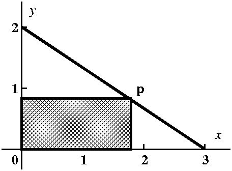 Probably the first thing I would do when meeting a problem of this
type is to draw a picture. I think my sketch would look something like
what's to the right. Certainly, I would need the line segment joining the points (3,0) and (0,2) in the
first quadrant which is drawn. Then I likely would try to draw
a typical rectangle. Although I tried to write the specification of
the rectangle in a direct way, my desire to be brief may have made
this difficult to understand. The rectangle has sides on the x- and y-axes as shown. It
also has a vertex on the line
segment. Legitimate questions include, "What's a vertex?" and
"What line segment?" I hope, even if you've not heard the word before
or this use of the word, that you would know "vertex" means a corner
of the rectangle. And the first sentence of the problem defines "the
line segment".
Almost surely in my mind I would play around with the problem as
pictured, and try to see some of the eligible rectangles. The pictures
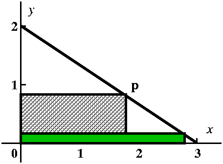
I would look at would include the two below. If the vertex were very
near (0,2), as in the left picture, I see that one side of the
rectangle would be almost 2 units long, while the other is very
small. The area of that rectangle would be small. On the other hand
(right picture), if the vertex were very near (3,0), one side of the
rectangle would be almost 3 units long, while the other is very
small. Again the area would be small. This encourages me to think
that, yes, there is a maximum and almost surely the max area will
occur for some rectangle with vertex "inside" the segment (at a
critical point of the algebraic model we will build).
| Two "extreme" rectangles |
|---|

Small area
|
Also small area
|
What to do ...
I mentioned in class that there is sort of a translation
process, going from the problem statement and creating a calculus
problem. I find this, even though I have a great deal of experience,
to be difficult. I generally need to read the problem statement very
carefully, and usually I need to read the statement several
times. Then there is an analysis step, where the calculus
problem is solved. This is usually more straightforward. It isn't
simple, because of course the opportunity for error is always present:
arithmetic errors, algebra errors, calculus errors. Certainly I have
made all of these, but somehow those can be fixed, at least for me,
more easily while the translation process definitely stubbornly proves
to be more difficult, at least for me.
Building the algebraic model
We will need the equation for the line segment. In class I tried to
describe how I would "guess" this equation. Since this is top secret
and also silly, I will just write it here: (x/3)+(y/2)=1. Well, o.k.,
my guessing method goes like this: the equation will involve both
variables since the line is neither vertical (x=const) nor horizontal
(y=const). Therefore it could be written
(x/something)+(y/something else)=1. Then plugging
in both (0,2) and (3,0) give me the values of something and
something else. What about the area of the rectangle? If
the coordinates of the point p are (x,y), then the area is xy.
I'm almost "there". The objective function is xy. The constraint
situation certainly involves (x/3)+(y/2)=1 but there is just a bit
more. Notice we are in the first quadrant, so that both x and y are
non-negative. Now my model follows:
Constraint(x/3)+(y/2)=1 and x≥0 and y≥0.
Objective Maximize xy.
As before I'll use the constraint to reduce the number of variables in
the objective. So (x/3)+(y/2)=1 becomes y=2[1–(x/3)] and xy becomes
2x(1–(x/3)). But don't forget the remainder of the constraint, which
becomes a domain restriction: x is in the interval [0,3].
The resulting calculus problem
Find the max value of f(x)=2x(1–(x/3)) when x is in the interval
[0,3]. We know that the maximum of f on [0,3] occurs either at
endpoints or critical points.
• Endpoint evaluation
f(0)=2·0(1–0)=0; f(3)=2·32(1–(3/3))=0. I bet
the max is inside, at a c.p.
• Critical point analysis Since
f(x)=2x(1–(x/3)) I know that
f´=2(1–(x/3))+2x(–1/3)=2–(4/3)x. Therefore the only c.p. is where
2–(4/3)x=0 so x must be 3/2. f(3/2)=2(3/2)(1–(1/2)) is positive, so
this is the maximum value. Yes, it "simplifies" to 3/2. The answer to
the problem is 3/2. Notice that the problem requests the largest area. We should attempt to answer
the question that is asked (so remarking that the dimensions of the
rectangle are ... and ... is not responsive!).
You should ...
Do 8 or 10 of these problems yourself, possibly together with other
students. Certainly what I wrote about is much more than I expect you
to write, but I would hope that, after sufficient experience,
you would think through such problems in much the same way as what's
above. I wanted to help you learn the process.
Practice is essential to your own ability to answer questions
of this type. The "translation" skill, that is, constructing the
correct mathematical model, is very important in applications.
A story about smallest
A line segment joins a point on the
positive x-axis with a point on the positive y-axis. The line segment
goes through the point (3,2) and creates, with the appropriate parts
of the x- and y-axes, a triangle. Find the smallest area of such a
triangle.
|
We discussed this a bit. We sketched the geometric situation
relatively quickly, but then students seem to have found making the
transition from the geometry to an algebraic description not so
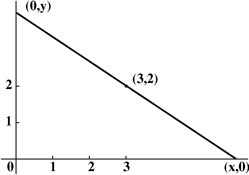
easy. There's a diagram to the right. It shows a "typical" line
segment which joins a point on the
positive x-axis with a point on the positive y-axis and which
also goes through the point
(3,2).
| 
|
As I wrote in a discussion of a previous geometric "story", I would
play around with the problem. When the point on the x-axis is very
close to (3,0), then the line would tilt "way up", very steeply. The
length of the line segment would be large and the area would be large
also (the length of the base →3 while the height →∞.
The area, which is (1/2)(base)(height) would therefore be large.
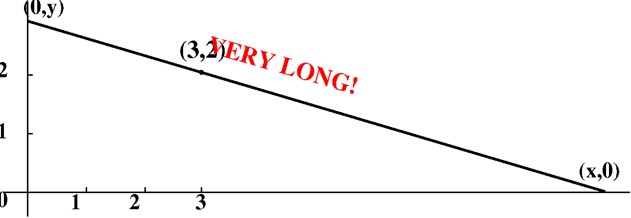
Similarly, if we were to pull the point on the x-axis far away from
(3,0), the slope would be close to 0, and the length of the line
segment would be large. The length of the base →∞ while the
height →∞. Again, the area would be large.
|  |
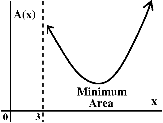 This seems to suggest that the area varies, and that "somewhere
in the middle" there is a minimum, and the minimum will occur at a
critical point. To the right is a very vague picture of x and A(x),
the area of the triangle when (x,0) is one end-point of the
segment. Here we note that the x's are in the interval (3,∞)
because otherwise we won't get a triangle -- the line segment won't
hit the positive y-axis. Also, I drew the graph so that as
x→3+ the area function gets very large, and a similar
behavior occurs as x→∞.
How about the transition from picture to an algebraic description? The
area is (1/2)xy, the Objective Function. How can we relate x and y
(the Constraint)?
If a diagram of the situation is labeled, then
some restrictions almost yell at the reader. Look to the right.
 Certainly x>3 and y>2. And there are bunch (well, three) similar
triangles which give some further relationships between the
variables. For example, the big triangle and the lower right small
triangle tell me that y/x=2/(x-3), so that y=(2x)/(x-3). And therefore
the function we need to minimize is f(x)=(1/2)(x)(2x)/(x-3). What is
the domain of this function when used to describe this problem?
Certainly, x>3. There is no other restriction. Now we have turned
this into a calculus problem.
A calculus problem
What is the minimum of f(x)=x2/(x-3) for 3<x<∞?
(I canceled the 2's and combined the x's.)
• Endpoint evaluation There are no
endpoints! But I would still begin with some sort of analysis or
understanding of what happens out towards the edges. So maybe I should
call this
Edge analysis What happens as
x→∞? Well,
limx→∞f(x)=limx→∞sqrt(x2/(x-3)].
When x gets very large, we have a degree 2 polynomial on top and just
a degree 1 polynomial on the bottom. We analyzed such situations
before, and the result is that x→∞.
Now what happens as x→3+? Well,
x2→32. But 1/(x-3) is like 1/(something small and
positive), which is large and positive. So I bet that the product of
these two →∞, just as we should expect from our previous
thoughts.
Comment I like the idea of wearing both belt and suspenders to
keep my pants from falling down. Well, maybe not exactly that, but I
certainly do like the idea of reinforcing my geometric understanding
of the problem with another, algebraic approach. Both methods should
be used! Also, this way, I can be sure that if we identify
critical points, the resulting value(s) of the function will include
the minimum, and won't be a maximum. As I mentioned in class, there
have been some interesting real world failures of engineering projects
where this identification (max vs min) was neglected.
• Critical point analysis If
f(x)=x2/(x-3) then
f´(x)=[(2x)(x-3)-(1)x2]/(x-3)2 (Quotient
Rule). Then f´(x)=0 when the top is 0, so we need to solve
2x(x-3)-(1)x2=0. We can factor this (it is a toy
problem!) and get x[2(x-3)-x]=0 which has roots x=0 (first factor) and
x=6 (second factor). We can discard 0 since that is not in the domain
for this problem. Therefore the minimum area occurs when x=6 (we only
know this is a minimum because we did the edge analysis,
otherwise we'd need more work), and f(6)=36/3=12.
Resembles...?
The last two stories had pictures which resembled each other quite a
bit. We minimized an area, and we maximized an area. The two problems
are actually related to each other. They are examples of what are
called dual problems. In economics, such problems occur when we
want to maximize profit. This might be the same as minimizing cost. In
physics, the ideas are minimizing work and maximizing potential
energy.
My darling, struggling in the ocean!
The last story for class.
I am standing on a straight beach
and my darling is swimming in the ocean, a quarter mile from
shore. The closest point to my darling is two miles down the
beach. The sharks attack, and I must get to my darling as soon as
possible. I can run a mile in 10 minutes and swim a mile in 40
minutes. How can I get to my darling in the least time?
| As I mentioned in class, this is actually not such a toy
problem. Similar problems arise in optics frequently: minimizing
travel time when the speed of light in different materials
varies. I've attempted to sketch the situation, as seen from "above".
How can I get from my initial position to my darling? | 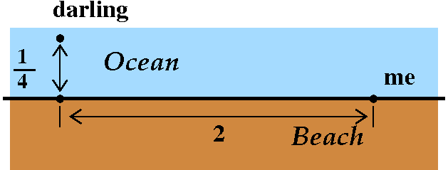 |
Pure strategy #1 Swim all the way!
Swim directly. The distance is sqrt((1/4)2+22),
about 2.01555 miles. At 40 minutes per mile, this takes about
80.6226 minutes. |
 |
Pure strategy #2 Run as much as possible.
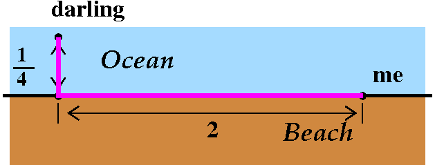
I run 2 miles down the beach, and then swim. So the 2 miles running
take me 20 minutes, and the 1/4 mile swimming takes 10 minutes. The
total time is 30 minutes. |
 |
A "mixed" strategy? Run for a while, then swim.
It is not clear but maybe some blend of the two is faster. So I
could run part of the way, and then swim directly to my darling. |
 |
|
Suppose
the "breakpoint" between these two activities is x miles from the
point on the beach which is closest to my darling. Then I'd run 2-x
miles, which would take 10(2-x) minutes. I would need to swim the
length of the hypotenuse of a triangle with legs x and 1/4 long:
that's sqrt(x2+(1/4)2) miles, and that would
take 40sqrt(x2+(1/4)2) minutes. The total time
would be f(x)=10(2-x)+40sqrt(x2+(1/4)2). The
domain of interest is [0,2]. |
 Amazing!!!
To the right is a fairly careful graph of f(x) (which I requested as
the QotD). Notice that there is a critical point in the
interval [0,2]. The critical point is close to 0. I used my "friend"
Maple to find the critical point. Partly
this is because I am lazy, but it is more because I am tired. This
computation could be done by hand, because the most "difficult"
part of it is just solving a quadratic question. The first instruction
defines f as the algebraic mess we have above. Maple echos the definition so that I can check
it is what I want (I make lots of typing errors!). The second
instruction differentiates this formula. The third instruction, which uses
the word solve, sets the previous
expression (that is what % means) equal
to 0. The answer is exact and comes from the quadratic formula. Then I
substituted this into the expression for
f. Since I didn't "understand" the expression, I used evalf to find a 10 digit approximation to the
answer.
 > f:=10*(2-x)+40*sqrt(x^2+(1/4)^2);
                                               2     1/2
                      f := 20 - 10 x + 10 (16 x  + 1)

> diff(f,x);
                                       160 x
                             -10 + --------------
                                        2     1/2
                                   (16 x  + 1)
> solve(%);
                                       1/2
                                     15
                                     -----
                                      60
> subs(x=%,f);
                                 1/2       1/2   1/2
                               15      2 16    15
                          20 - ----- + -------------
                                 6           3
> evalf(%);
                                  29.68245837
At the all swimming endpoint, the time needed was about 80.6226
minutes. At the most running endpoint, the time needed was 30
minutes. The ideal strategy (at least for minizing time!) gets me to
my darling in less time than that: 29.6824 ... minutes.
I will certainly happily admit that this is not a great difference in
time. But you should see that there is a difference, and in
other problems the difference might be significant.
The speed of light in vacuum (air is about the same) is
299,792,458 meters per second (I copied this!). This speed is
frequently called c. "Denser media, such
as water and glass, can slow light much more, to fractions such as 3/4
and 2/3 of c." This difference is responsible for light "bending"
or refracting, because light travels (!) to minimize time.
|
L'Hôp
This is the next topic in the syllabus. L'Hôpital's (also
L'Hopital's or L'Hospital's) Rule is a method of evaluating certain
very special limits. It is worth showing to you because it is another
neat application of "local linearization", and some really important
limits become easy to evaluate. However, it must be used with some
care. One
quote I found on the Internet declared, "Giving l'Hopital's Rule
to a calculus student is like handing a chainsaw to a three year old."
The example I was going to begin with is
limx→0[sin(9x)/(e6x-1)]. "Plugging in" gets
no information, since we have 0/0. By the way, 0/0 limits can have
strange and varied behavior. For example, consider as x→0 the
three expressions x2/x and x/x and x/x2. They
all result in 0/0 when we just plug in. But if you think about them a
bit, the first has limit=0, the second has limit=1, and the limit for
the third expression does not exist. So 0/0 can conceal lots of
different behaviors.
You'll learn more about L'H on Monday.
| Tuesday, November
3 | (Lecture
#18) |
|---|
Exam warning!!!
The second in-class exam will be given Thursday, November 19, at the
usual class time and place. More information will be available
soon. Pleased study carefully.
Graphing a function
I gave data about a function in a rather strange way.
- f is a differentiable function whose domain is all real
numbers except for –2 and 1.
- f´ is positive only in the intervals x>3 and
–2<x<0.
- These limits are known:
limx→1–f(x)=–∞;
limx→1+f(x)=+∞;
limx→–2+f(x)=–∞;
limx→–2–f(x)=–∞;
limx→+∞f(x)=–1;
limx→–∞f(x)=0.
This is a great deal of mostly "qualitative" information (the
limits). I'm not giving any specific values of f, for example. I aimed
at drawing a qualitatively correct graph, but did admit that I
could "predict" how big f(3) was, for example.
Thinking about the graph of y=f(x)
The process is important. I'll try to go slowly through every bit of
information. I may make mistakes, and I may have to fix things
up. I'll only be able to sketch somethng which is qualitatively
correct.
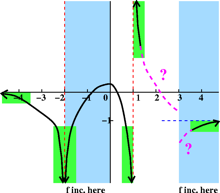
|
Fact f is a differentiable function whose domain is all real
numbers except for –2 and 1.
Response I'd probably try to indicate somehow to myself that
the graph I'll draw should not appear when x=–2 and on x=1.
| 
|
|
|
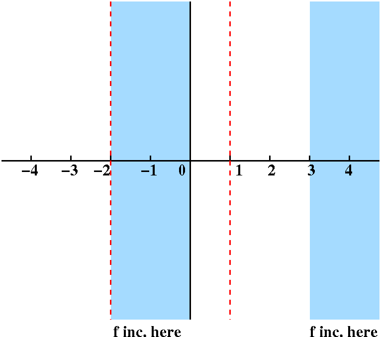
Fact f´ is positive only in the intervals x>3 and
–2<x<0.
Response f is increasing in those intervals where the
derivative is positive. An important word in the "Fact" sentence is
only. To me this says that f is increasing only in the
intervals from –2 to 0 and from 3 upwards. In interval notation, these
are (–2,0) and (3,∞). Probably f will be decreasing
in other intervals.
| 
|
|
|
Fact limx→1–f(x)=–∞.
Response The symbols x→1– mean x is getting
close to 1 from the negative (left) side. And then –∞ means
that f(x) is getting large, but large negative, so the graph is going
down. What I would expect is something like what is shown here.
| 
|
|
|
Fact limx→1+f(x)=+∞.
Response Here we have x→1+ and we should
consider x getting close to 1 from the right, positive side. The
+∞ means that f(x) will be getting very large positive. The
direction of approach and the largeness combine to get a sort of piece
of a graph which looks like what is shown.
| 
|
|
|
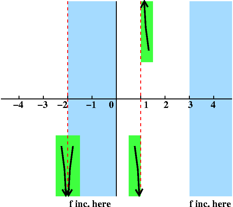
Fact
limx→–2+f(x)=–∞;
limx→–2–f(x)=–∞.
Response I'll do these next two as a pair. The notation is
somewhat intricate here. We've got x→–2+ and
x→–2–. So x is getting close to –2 from the
right (+) and from the left (–). The result in both cases is
–∞. The f(x) is getting large negative as x gets close to –2.
| 
|
|
|
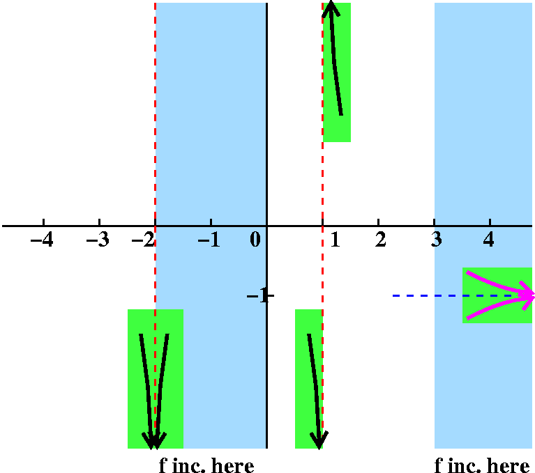
Fact limx→+∞f(x)=–1.
Response This is new (at least in the lectures). The
x→+∞ indicates the idea that x is traveling far to the
right. As it does, f(x), the y coordinate on the graph, is getting
close to –1. I don't really know exactly what I should draw.
I drew two possible candidate graphs in magenta. Both of the pieces of curves drawn
satisfy the limit statement (there are, as I mentioned, even other
possibilities to draw). BUT we can select exactly one as a
valid candidate using other information. This piece of y=f(x) is drawn
in a region where the derivative is positive, so the graph should be
increasing. Therefore we can drop the top candidate and the other,
wiggly (?) possibilities.
| 
|
|
|
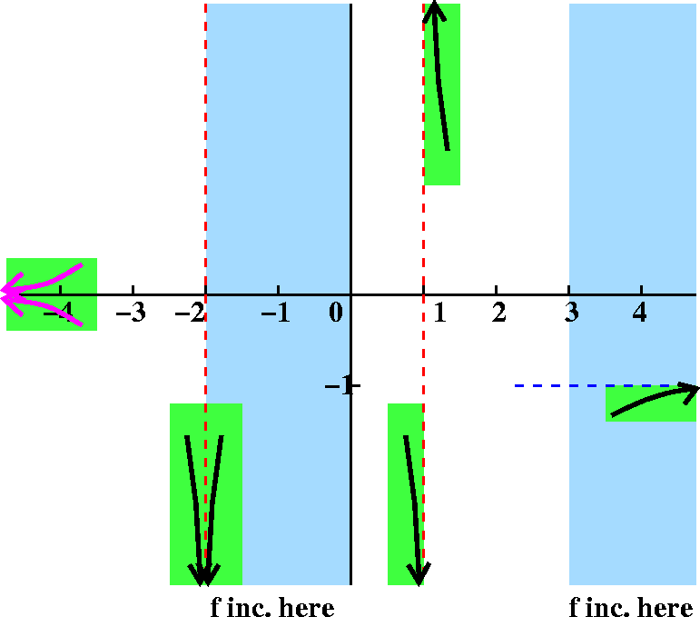
Fact limx→–∞f(x)=0.
Response We've gotten to the final limit statement. Here
x→–∞ means that x is moving "far" to the left. And
the =0 tells me that the graph is getting close to the x-axis. Again
I've drawn two possible candidates. Which one will be appropriate?
Here we need knowledge once more about {in|de}creasing behavior to
make a selection. We are outside of the region where we know
f(x) is increasing, and since we had that word "only" we should expect
in this region that f(x) is decreasing. The lower alternative, the
bottom candidate, is the one we should select.
Please note that in the behavior on the right, I have drawn only the
surviving candidate as supported by the previous picture's discussion.
| 
|
|
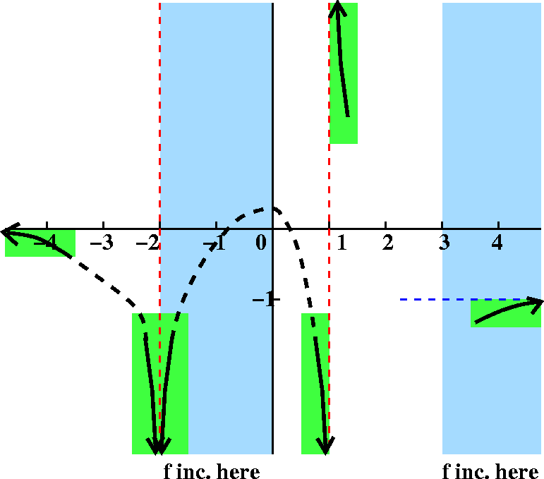
Further discussion
We've got to complete the graph. Let me move from left to right. I
know that the graph must be differentiable and therefore also
continuous. In the region to the left of –2, I think the graph
should be decreasing. I have indicated a tentative way of joining the
two pieces we've already drawn, and you should check that what's
suggested is indeed decreasing.
Now consider the region between –2 and 1. This is a bit more
complicated. We need to be increasing until 0, and then,
probably, decreasing. And we should draw a continuous graph which
connects what the limit statements gave us. So I have tried to suggest
a good candidate. Notice, please, that although I am fairly sure f has
a local maximum when x=0, I really have no idea where the local
maximum is (I don't even know if the value is positive or
negative). I've only been given qualitative information. So my
suggestion is only one of many which would be consistent with what's
required.
| 
|
|
And more discussion
What happens between 1 and 4 in the picture? To the right of 3, that
is, for x>3, f should be increasing. So we guess something like the
magenta piece shown. And to the left of 3,
in the region with 1<x<3, we know that f is not
increasing, so probably (!) it should be decreasing. The result
could be what is shown in this magenta piece. but I've inserted large question
marks because something strange has happened: if we accept both
suggestions as drawn the result will certainly not be
continuous.
The graph should not have a jump in it. How can we fix this?
You need to think a bit.
| 
|
|
The last piece
A curve which completes the graph validly, satisfying all of the
specifications, is shown to the right. From 1 to 3, the graph
decreases, dropping below the horizontal asymptote y=–1. Then,
at x=3, the curve begins increasing, and blends into the required
asymptotic behavior as x→+∞.
This graph has two vertical
asymptotes (x=–2 and x=1) and two horizontal asymptotes (y=0 and
y=–1).
To the right is sketched one correct answer to this problem. Again,
the problem is mostly qualitative, and there could be many specific
graphs which are correct answers to the problem. I do know that for
any solution to this problem, there will be two critical
points. There will be one at 0 which will be a local max, and there
will be one at 3 which will be a local min. Additionally, there will
be at least one inflection point, somewhere to the right of 3. (As I
mentioned in class, we could imagine the curve wiggling a bit, not
changing its {in|de}creasing behavior, so I can't declare that there
will be only one inflection point -- there will be at least
one.)
| 
|
|
Comment
I began the "construction" of the previous problem by sketching a
graph and working backwards. I "read off" the limit statements from
the graph. If you just wrote limit statements at random without
starting from information that you knew was consistent, the resulting
specifications might be impossible to fulfill. Also, I really believe
I could create a function defined by an algebraic formula which had a
graph similar to what was drawn above.
Limits at +/–∞
I wanted to give examples of some of the algebraic manipulations
resulting in horizontal asysmptotes which you should know about. So
here they are.
3. What is
limx→∞[8x5–5x3+88x]/[x4+3x+9]?
In this case the degree of the top is one greater than the
degree of the bottom. Dividing the top and bottom by x4 gives
[8x–{5/x}+{88/x3}]/[1+{3/x3}+{9/x4}].
The bottom is 1+{3/x3}+{9/x4} and I think as
x→∞ the bottom gets close to 1 rather rapidly.
The top is [8x–{5/x}+{88/x3}. The second and third terms
are negligible as x gets large, and the top seems to be nearly 8x. I
think that the quotient will behave as 8x/1 for large x, and the limit
will be ∞.
A graph is shown to the right. Please notice that in this case, x goes
from 0 to 10 and y, from 0 to 80. The graph appears to resemble
closely a straight line of slope 8, which is what the algebraic
manipulation suggests.
|  |
A weird one ...
I also consider the function f(x)=(5x+7)/sqrt(x2+3). Here
let me begin by displaying a graph, since the algebraic
analysis did not proceed very well in class. Below is a graph of
y=f(x) for x between –30 and 30. Also on display (the dashed green lines) are the horizontal lines y=5 and
y=–5. Look at the graph, and observe (I hope!) that the limit as x
gets large positive of f(x) seems to be 5, and the limit as x gets
large negative of f(x) seems to be –5. The situation is more
complicated than the previous examples.

What's happening? Look at sqrt(x2+5) and "massage" it
algebraically. Well, sqrt(x2+5)=sqrt(x2·(1+{5/x2})).
| Square root facts |
|---|
The function which is sqrt
Sqrt is a function whose domain is [0,∞) and whose
range is [0,∞).
Example The value of sqrt(4) is 2. The equation x2=4
has two roots. We could indicate these two roots by writing
+/–sqrt(4), but sqrt(4) without any "decoration" always means 2. |
Multiplication works well
sqrt(A·B)=sqrt(A)·sqrt(B) if both A and B are
non-negative.
Example
sqrt(400)=sqrt(4·100)=sqrt(4)·sqrt(100)=2·10=20. |
Addition does not work with square root
There is no simple relationship between sqrt(A+B) and sqrt(A)+sqrt(B).
Example sqrt(25)=5 and sqrt(16)=4 and sqrt(9)=3. Although
16+9=25, notice that 3+4=7 which is not equal to 5.
That is: sqrt(16+9) and sqrt(16)+sqrt(9) are very different. |
Therefore sqrt(x2·(1+{5/x2})) is the same as
sqrt(x2)·sqrt(1+{5/x2}).
Please notice that if x>0, then sqrt(x2) is the same as
x. So:
If x>0 then
f(x)=(5x+7)/sqrt(x2+3)=(5x+7)/[x·sqrt(1+{5/x2})].
Divide the top and bottom by x and the result is
(5+{7/x})/[sqrt(1+{5/x2})] and I hope that now you can see
the limit as x→∞ is 5.
If x<0 then sqrt(x2) is the same as –x. You
can check this: try, say, x=–5 and see what happens. So look at
f(x):
f(x)=(5x+7)/sqrt(x2+3)=(5x+7)/[–x·sqrt(1+{5/x2})].
Dividing top and bottom by x gets
(5+{7/x})/[–sqrt(1+{5/x2})]. As
x→–∞, this becomes –5.
 Damped oscillation
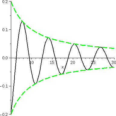
The function f(x)=sin(x)/x is actually something I'm more comfortable
discussing with engineering students, since things that it "models"
are easily observed. As x→∞, the bottom, x, grows, and the
top, sin(x), is caught between –1 and 1. This function should approach
0. In fact, an appropriate version of the Sandwich Theorem can
be used. By this I mean, please, just realize that:
–1/x≤sin(x)/x≤1/x.
Since both –1/x and 1/x →0 as x→∞ f(x), which is
caught in between, also approaches 0.
A graph of y=f(x) is shown to the right. The "envelope curves",
y=+/–1/x, are dashed green curves. You will
study oscillations whose amplitude go to 0 (think of a spring
vibrating in a viscous fluid).
|
A story about numbers
The sum of two non-negative numbers is 20. How
should the numbers be selected so that the product of the square of
one with the other is largest?
We should translate this problem statement into algebra, and then we
will use methods of calculus to solve the problem. This is a "toy"
problem, but the process remains valid even in much more complicated
situations. The translation is important. We may not always be able to
solve a problem, but calculus can usually move the analysis of the
problem closer to a solution.
So the two non-negative numbers will be
called x and y. We know that x≥0 and y≥0. We also know that
their sum ... is 20 so x+y=20.
We want to know How should the numbers be
selected to make something largest. What's the quantity we should try to
maximize? It is the product of the square of
one with the other and this is, I think, x2y.
The problem can be translated to the following algebraic statement:
Suppose x+y=20 and x≥0 and y≥0. Find the maximum value of
x2y.
In economics and some other disciplines, the first sentence is called
the constraint. It relates the variables of the problem and
restricts which values should be considered. It usually is related to
the appropriate domain of the problem. The second sentence is the
objective function. It describes what should be "extremized" --
in this case, what should be maximized or made largest. Here the
objective involves two variables, x and y. But the constraint tells us
that y=20–x. And therefore the problem description changes.
Suppose f(x)=x2(20–x). The domain for this problem is
[0,20]. How can we get the largest value of f?
Notice that the constraint, which shouldn't be forgotten, has
resulted in the domain statement when we write this version of the problem.
Now we can use calculus. The maximum of f on [0,20] occurs either at
endpoints or critical points.
• Endpoint evaluation
f(0)=02(20–0)=0; f(20)=(20)2(20–20)=0. I bet the
max is inside, at a c.p.
• Critical point analysis If
f(x)=x2(20–x), then f´(x)=2x(20–x)–x2. This
is 0 when =2x(20–x)–x2=0 or x(40–2x–x)=0 or x(40–3x)=0. So
we get x=0 (already checked) and x=40/3. Since
f(40/3)=(40/3)2(20–40/3) is positive (20 is 60/3),
this is where the max value of f occurs.
The answer to the question is 40/3 and 20–40/3 (we were asked
How should the numbers be selected).
Another story
A line
segment joins the points (3,0) and (0,2) in the first quadrant. A
rectangle in the first quadrant which has sides on the x- and y-axes
is inside the resulting triangle, and has a vertex on the line
segment. What is the largest area that such a rectangle can
have?
Comment
I really tried to write the specifications in this problem
carefully. After class, Mr. Orrico and
Ms. O'Sullivan convinced me that my
paragraph was not carefully written enough. I think they were
correct. Instead of the phrase "which has sides on the x- and y-axes
is inside the resulting triangle, and has a vertex on the line
segment", I had written "has sides on the x- and y-axes and a vertex
on the line segment". In that case (future lawyers should follow this
carefully!) a rectangle with vertices at (0,0), (3,0), (3,2), and
(0,2), that is a rectangle with the line segment as a diagonal, will
definitely have (I think!) all the other "eligible" rectangles inside
it. So it would definitely be the largest. This isn't what I
wanted. So my specification was not written precisely enough. I am
sorry. I believe (currently, about 5 hours later!) that what I've
written above is what I wanted and really do want. Sigh.
I will continue the discussion with the changed specification written
above.
 Probably the first thing I would do when meeting a problem of this
type is to draw a picture. I think my sketch would look something like
what's to the right. Certainly, I would need the line segment joins the points (3,0) and (0,2) in the
first quadrant which is drawn. Then I likely would try to draw
a typical rectangle. Although I tried to write the specification of
the rectangle in a direct way, my desire to be brief may have made
this difficult to understand. The rectangle has sides on the x- and y-axes as shown. It
also has a vertex on the line
segment. Legitimate questions include, "What's a vertex?" and
"What line segment?" I hope, even if you've not heard the word before
or this use of the word, that you would know "vertex" means a corner
of the rectangle. And the first sentence of the problem defines "the
line segment".
Almost surely in my mind I would play around with the problem as
pictured, and try to see some of the eligible rectangles. The pictures
I would look at would include the two below. If the vertex were very
near (0,2), as in the left picture, I see that one side of the
rectangle would be almost 2 units long, while the other is very
small. The area of that rectangle would be small. On the other hand
(right picture), if the vertex were very near (3,0), one side of the
rectangle would be almost 3 units long, while the other is very
small. Again the area would be small. This encourages me to think
that, yes, there is a maximum and almost surely the max area will
occur for some rectangle with vertex "inside" the segment (at a
critical point of the algebraic model we will build).
| Two "extreme" rectangles |
|---|

Small area
|

Also small area
|
I will finish this problem on Thursday and discuss some additional problems.
| Thursday,
October 29 | (Lecture #17) |
|---|
What first derivatives can tell you
We learned last time:
- If f´>0 on an interval, f is increasing
on that interval. Therefore if you "move" from left to right on the
graph, you'll also move up.
- If f´<0 on an interval, f is decreasing
on that interval. Now if you "move" from left to right on the
graph, you'll move down.
What second derivatives can tell you
The sign of the second derivative on an interval also has some neat
geometric information. Here is the logic:
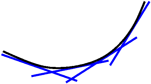
If f´´>0 on an interval then f´ is increasing
on that interval. So moving from left to right means that the slope of
the tangent line increases. I don't know enough about animations to
put my walking demonstration of this on the web (I wish I did, but I
am lazy), but to the right is a static picture of what I am trying to
describe. This curve is concave up.
 Of course, if f´´<0 on an interval then f´ is
decreasing on that interval. So moving from left to right means
that the slope of the tangent line decreases. A typical geometric
picture of this situation is to the right. (Since I am lazy, all I did
was flip the previous picture -- drawing programs are wonderful.)
This curve is concave down.
The Second Derivative Zoo
Before we went on, I thought giving several (relatively) simple
examples would be useful. I learn far more from examples than from
definitions, and even from theorems. So here is my "zoo" or collection
of concavity examples.
| Examples and discussion | Graphs |
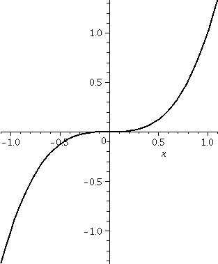
|---|
| x3
Here f(x)=x3 so f´(x)=3x2. Away from x=0,
this is certainly positive, so f is increasing in (–∞,0] and in
[0,∞). Actually, if we "glue" the intervals together, we can
see that f is increasing in all of the real numbers.
Since f´´(x)=6x, I know that f is concave up where
6x>0: this is (0,∞). Similarly, f is concave down
where 6x<0. This is (–∞,0).
At 0, the x-axis (equation:y=0) is a horizontal tangent line. Also at
x=0, the concavity changes from down to up. This is called an
inflection point.
|  |
| x1/3
Well, this function is a bit weirder. Here
f´(x)=(1/3)x–2/3. You need to think about this for a
moment. The derivative is a negative power of x. This means
that the domain of the derivative does not include 0 (we don't divide
by 0!). Geometrically, this function is the flip over the "main
diagonal" y=x of y=x3: it is the inverse of
x1/3. The previous horizontal tangent line becomes a
vertical line, which has no slope. Since
=(1/3)x–2/3=(1/3)(1/x2)1/3, I know that the derivative (where it
exists!) is always positive. This function is increasing always.
Since f´(x)=(1/3)x–2/3, we know that
f´´(x)=–(4/9)x–5/3. Again, the domain is non-zero
x's. But what is the sign of f´´(x) for those non-zero x's?
Here please notice that 5 and 3 are both odd. This is important. A
negative number raised to an odd integer power or an odd integer root
is negative. But look closely: in front of the formula, before the
(4/9) is –: a minus sign. So f´´ is positive
when x is negative, and therefore the graph is concave up for
negative x. For similar reasons, the graph is concave down when x is
positive. And x=0 is a point on the graph where concavity changes, and
therefore is an inflection point.
|  |
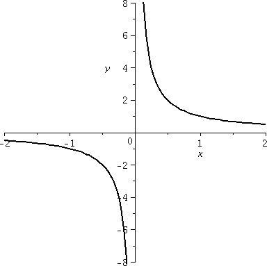
| 1/x
There is a tricky bit of language here, which I will mention
later. Since f(x)=1/x=x–1, I know the
f´(x)=–1/x2. Squares are always positive, so this
derivative is always negative, and therefore, inside each interval
in which this function is defined, the function is decreasing.
This means f is decreasing inside (–∞,0) and f is decreasing
inside (0,∞). Notice, though, that f(1)=1 and f(01)=–1. Even
though –1<1, we have f(–1)<f(1): f is not decreasing "across"
the intervals.
If we compute correctly, f´´(x)=2/x3. 3 is an
odd power, so the graph is concave down in (–∞,0) and concave
up in (0,∞). The domain of f does not include 0, so
there is no point of inflection!
|
 |
|
|x|
I put this in to stimulate some conversation. If you are clever and
just look at the graph, you can "read" the derivative. The function
f(x)=|x| is differentiable except for x=0. When x<0, f´(x)=–1,
and when x>0, f´(x)=1. Actually, the second derivative also
"exists" when x is not 0: f´´(x)=0 for all x not equal to
0. The graph has no concavity as it is usually understood.
|  |
| x4
If f(x)=x4, then f´(x)=4x3 and
f´´(x)=12x2. If x is not equal to 0, then
the second derivative is positive. The graph is concave up. Notice
that although f´´(0)=0, this graph has no point of
inflection! The concavity on both sides of x=0 is "up": the graph is
concave up in both (–∞,0) and (0,∞). Since concavity
is the same on both sides of 0, the origin is not a point of
inflection.
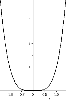
 Comment
People will say that y=x4 "is" or "looks
like" a parabola. Well, right here (to the right, here!) are graphs of
y=x2 and y=x4. I will agree that the graphs
resemble each other in many ways. They are both concave up always, go
through (0,0), and are symmetric with respect to the y-axis. But
please look a bit more closely. y=x4
is flatter near the origin (higher powers of small numbers are
smaller!). As soon as the x's get out of [–1,1], that curve grows much
larger than y=x2 (higher powers of
large numbers are larger). The parabola is y=x2 and it has
some interesting geometric and physical properties (for example,
mirrors are made to have parabolic cross-section to help aim light
beams and telescopes) which are not shared by y=x4.
| 
|
Inflection point
x is an inflection point of f if
- x is in the domain of f.
- The concavity of the graph of f on the two sides of x (less than
and greater than) is different.
Templates (pieces of curves) based on signs of f´ and
f´´
The QotD was to fill in curves in the four spaces in the table below
this paragraph. Each space was supposed to be a small segment of a
curve which characteristically looked like the properties which define
its place in the table: So {in|de}creasing and concave {up|down} are
these properties and most students seemed to fill in the blanks
correctly. The little chunks (?) of these curves can be used to
"build" more complicated curves.

 The Gaussian (bell-shaped) curve
I wanted to graph a "random" (not!) curve defined by a formula. What
we looked at was f(x)= e(–x2). This turns out to
be a rather important function in analyzing experimental
results. Any "real" repeatable experiment with a measurable
outcome is likely to have the numbers scattered so they resemble
this bell-shaped curve. This phenomenon is not obvious at all!!
The exponential function's outputs are never negative and never
0. Therefore no part of the graph will be on or below the
x-axis. Since –x2 is always less than or equal to 0, and
these numbers serve as inputs to exp, I bet that the outputs from exp
will be less than or equal to 1, and will be equal to 1 only at
x=0. Also this graph is even, symmetric with respect to the x-axis,
since (–x)2=x2. I hope this explains to you why
the graph looks the way it does. But let me try analyzing the graph
using the first and second derivative.
If f(x)=e–x2 then
f´(x)=(e–x2)(–2x). The exponential function is
very nice. It is never 0 and always positive. Therefore the
only x for which f´(x)=0 is when –2x=0. So x=0 is the only
critical number. Now reasoning using the Intermediate Value Theorem
says that f (which is certainly continuous!) can have only one sign
for x<0 and one sign for x>0 (or else f(x) would have to have to
be 0 again). We can check signs at, say, x=1 (where the derivative is
negative) and x=–1 (where the derivative is positive). f is increasing
in (–∞,0) and f is decreasing in (0,∞). Naturally 0
represents a local (and indeed, absolute!) maximum.
What information can we get from the second derivative? If we use the
product and the chain rule correctly, then
f´´(x)=(e–x2)(4x2–2). Logic
similar to the preceding asserts that this is 0 exactly when the
non-exponential factor is 0. But 4x2–2=0 when
x={+|–}1/sqrt(2). Again, we can check signs in between the 0's of f'',
and f will be concave up for x<–1/sqrt(2) and for
x>1/sqrt(2). For x between –1/sqrt(2) and +1/sqrt(2), the graph
will be concave down. The points where x={+|–}1/sqrt(2) are where the
concavity of f changes: these are called inflection
points. These particular inflection points are related to the
standard deviation, which represents dispersal from an average when
this function is used in statistics. The center of the curve, at x=0,
is related to the mean of the data observed.
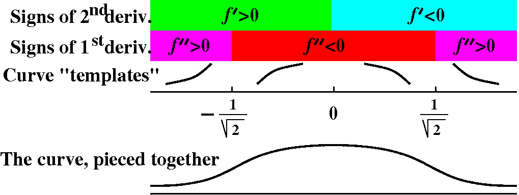
The diagram/picture above is an attempt to indicate how a person could
assemble the information about signs of the first and second
derivative, and patch together template pieces. The patched-together
curve should be continuous (no breaks) and differentiable
(smooth). This all takes some practice!
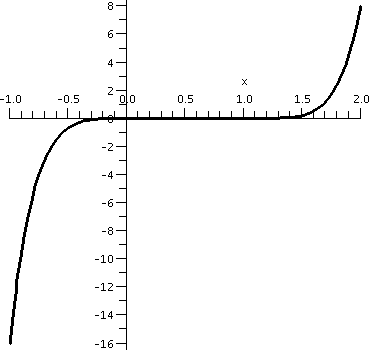 Graphing x3(x–1)4
Here I invited students again to use a graphing calculator and try to
see what y=x3(x–1)4 "looked like". I did remark
that the "action" took place somewhere between –1 and 2. The result of
this was something like the graph shown to the right. I believe that
calculators and graphing devices are wonderful, but sometimes they
almost conceal what's going on.
Here f(x)=x3(x–1)4. If we want to find out where
f is increasing and decreasing, we really should look at
f´(x). For this we need the product rule and the chain rule. So:
f´(x)=3x2(x–1)4+x34(x–1)3.
Generally I am against "simplifying" because I view it as mostly a
chance to make lots of mistakes. But here some simplifying will reveal
structure in the derivative. So please notice the common factors, and
what you get is as follows:
f´(x)=x2(x–1)3(3(x–1)+4x)=x2(x–1)3(7x–3).
What can we tell about where the derivative is 0 and where it is
positive and where it is negative? Well, the different factors allow
us to deduce that the derivative is 0 at x=0 and x=1 and x=3/7.
If x is very large positive, say, then f(x) is a product of three
factors, all of which are positive. And if x is very large negative,
then the x2 is positive and the (x–1)3 is
negative and the 7x–3 is negative. Therefore f(x) in that range is
positive also. So we have learned (using logic from the Intermediate
Value Theorem as before) that the derivative is positive on at least
the intervals (–∞,0) and (1,∞). There is a chance
for the derivative to change signs at x=0, but the factor which
controls sign change there is x2: since 2 is even, there is
no sign change at x=0. But there is a sign change at x=3/7 and at
x=1. So now we have broken up the real line into pieces based on
the signs of the derivative of f:
    Deriv is +     Still +          Now it is –        Back to + here
<---------------0-----------3/7--------------------1------------------->
 Func increases   increases     The func decreases   Here it decreases
|
So from this I learn that f has critical points at 0 and 3/7 and 1. We
can also learn that f has a local max at 3/7 and a local min at
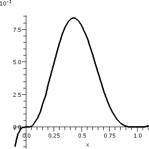
1. This is not entirely clear from the initial graph. Actually,
if we just look at the graph from –.1 to 1.1, you can see some of the
structure. This is shown to the right. Please notice that the vertical
scale of this graph is very small. This might all be difficult to see
without looking at the calculus first.
|
 |
Let's consider the concavity of this function, and make some
guesses about the number and location of inflection points. We can be
sure about this if we find the second derivative.
I will use the product rule, and make the second factor, a product
itself. So:
f´(x)=x2(x–1)3(7x–3)=
x2((x–1)3(7x–3))
f´´(x)=2x((x–1)3(7x–3))+x2(3(x–1)2(7x–3)+(x–1)3(7))
So let me try to "simplify" f´´(x). We will get:
x(x–1)2(2(x–1)(7x–3)+3x(7x–3)+x(x–1)7)=
x(x–1)2(2(7x2–10x+3)+21x2–9x+7x2–7x)=x(x–1)2(42x2–36x+6)
So the second derivative is 0 at x=0 and at x=1 and at the roots of
42x2–36x+6=0: those are x=(3/7)+/–sqrt(2)/7 (approximately
.227 and .631). The second derivative does not change sign at 1
because the factor is (x–1)2, an even power. It does
change sign at 0 and the two other numbers which are on either side of
the local max. There are three inflection points.
I needed to work fairly hard to get everything correct in the preceding
example.
Second Derivative Test
There is a result which allows you to tell when a critical point is a
local max or local min if you have information about the second
derivative at that point. It goes like this:
|
If f´(x)=0, and if f´´(x)>0,
then f has a local min at x. Example –x2 at 0.
| |
If f´(x)=0, and if f´´(x)>0,
then f has a local min at x. Example x2 at 0.
| |
If f´(x)=0, and if f´´(x)=0,
then nothing can be deduced. Example –x4,
x4, and x3 at 0.
|
I don't often use this result, because I am lazy and computing the
second derivative (and evaluating it!) may be work. Usually I can
examine the first derivative, if needed.
Inflection points as you drive!
 Suppose you are driving along a road, which happens to be the graph of
a function. Please refer to the picture to the right. This discussion
is an effort to persuade you that inflection "occurs" in the "real
world". My car is the weird object shown at the lower left, and it is
moving in the direction of the red arrow. This is a one-way road and I
won't hit anything (I hope).
As I drive along the road, I steer to the left (that's the A region of
the road). Eventually I come to a place where the road begins to
bend the other way, at B. After that point, in the C region, I
steer right. The bending place, where the switch from left steering to
right steering occurs, is an inflection point.
Please notice that from the point of view of the car, it actually
doesn't matter (no gravity, we are looking from above) whether the
curve is decreasing or increasing. The steering occurs as a response
to how the curve is bending. When the bending changes (inflection!) we
must change steering direction -- if we want to stay on the road,
anyway.
What could have been the QotD
 To the right is shown a graph of the derivative of
f(x). The function is intended to have domain all of R, the
real numbers, and the arrows at the end of the graph are intended to
indicate that the graph goes on forever behaving nicely. Please answer
the questions in A first, and then draw the graph requested in B.
A. Use this graph to answer the following questions as well as you
can.
- What are the critical points of f?
- In what intervals is f decreasing?
- In what intervals is f increasing?
- For each critical point: is it a local max or a local min or
neither?
- Where is the graph of f concave up?
- Where is the graph of f concave down?
- Where are the inflection points of f?
B. Sketch a graph of y=f(x) using the information just
described.
There will be many different valid graphs, but they will all share the
same qualitative features.
Please try to write a solution on your own. Then you may wish to look
at a solution I wrote.. Do this yourself
first, please. This is a valid exam question, and you should
check your own ability with such material.
|
| Tuesday,
October 27 | (Lecture #16) |
|---|
Two "easy" exercises
Two eager volunteers, Mr. Kadriu and Mr. Thistle, did the first problem
below. At the same time, eager volunteers Mr. Patel and Mr. Montero
did the second problem.
- Problem 53 of section 4.2 Find the max and min values of
f(x)=(ln(x))/x on the interval [1,3].
Endpoints f(1)=ln(1)/1=0 and f(3)=ln(3)/3.
The derivative
f´(x)=[(1/x)(x)–1·ln(x)]/x2. The top is
1–ln(x), and this is 0 when ln(x)=1, so x=e.
Plugging in f(e)=ln(e)/e=1/e.
Biggest/smallest of the available candidates Max must be 1/e and min
must be 0.

Comment We needed to compute 1/e: its decimal expansion begins
.3678, and ln(3)/3: its decimal expansion begins .3662. I certainly
can't "see" which number is larger. And, really the graph hardly
helps. (Later in this lecture we'll see another way to detect the
highest point without extensive computation.)
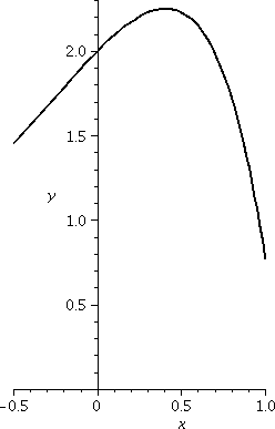
- Problem 54 of section 4.2 Find the max and min values of
f(x)=3ex–e2x on the interval [–1/2,1].
Endpoints f(–1/2)=3e–1/2–e–1 and
f(1)=3e–e2.
The derivative f´(x)=3ex–2e2x. When
is this 0? Well, we can factor:
ex(3–2ex)=0. Since ex is never 0,
this is 0 when 3–2ex=0 so ex=3/2 and x=ln(3/2).
Plugging in
f(ln(3/2))=3eln(3/2)–e2ln(3/2)=3(3/2)–(9/4)=9/4.
Biggest/smallest of the available candidates Max must be 9/4 and min
must be 3e–e2.
Comment Again, you can compute to compare the three values, or,
in this case, maybe the comparison can be done by "pure thought". So,
for example, f(1)=3e–e2=(3–e)e is about .3(2.7),
approximately .8 And f(1/2)=3e–1/2–e–1 is about
3/2–1/3, which is 7/6. And the other value is 9/4. So the 9/4 is
largest, and the (approximately) .8 is smallest.
What should you learn?
I do not think that that finding the max or min of even these rather
simple "toy" examples is totally straightforward. I don't think that
the answers can be guessed, even for these examples. And just trying
numbers at random is quite wasteful and would qualify as a stupid
strategy. The method outlined really works!
Rolle's Theorem
 If f is continuous on[a,b], and if f(a)=0 and f(b)=0, and if f is
differentiable inside the interval, then there is at least one number
c inside the interval where f´(c)=0.
To the right is a typical picture of the situation described in
Rolle's Theorem. Since the function is glued down (?) on the x-axis at
a and b, either the function is always 0 (so there are lots of c's) or
the absolute max and absolute min occur inside the interval. There may
be more than one of each. Since the function is differentiable, these
max's and min's occur at critical points where the derivative is 0, as
shown.
Below is a gallery of possible "Rolle" situations. The first, to the
left, is the simplest and silliest. The function is 0 in the whole
interval. Then any c is a valid candidate for the consequence of the
theorem. The second picture shows what happens if f is positive
somewhere. Then the absolute max must occur inside, and it must occur
at a local max inside the interval, and since f is differentiable,
f´(c)=0 there. The next is the negative situation, and the last
picture is what might happen if there f had a mixed sign behavior.

Rolle's Theorem tilted
Rolle's Theorem seems very specialized. What would happen if we tilted it?
That is, we took the coordinate axes and rotated the whole picture?
Then the graph is no longer glued down at the endpoints. This is the
important generalization that people use constantly. Of course, the
picture is relabeled and everything is more conventionally drawn.

Here is one of the two results in this course that anyone who
uses calculus will think about quite frequently.
The Mean Value Theorem (MVT)
 Suppose f is differentiable in [a,b]. Then there is at least one c
inside the interval so that f´(c)=(f(b)–f(a))/(b–a).
Discussion To the right is a tilted and relabeled picture. The
line segment joining (a,f(a)) and (b,f(b)) has slope equal to
(f(b)–f(a))/(b–a). The other indicated line segments are pieces of
tangent lines which are parallel to the segment joining (a,f(a)) and
(b,f(b)). Since they are parallel, their slopes must be equal. But the
slope of a tangent line at c is f´(c), and that's the equation
which appears above.
If you want an algebraic verification of MVT, then look at the end of
section 4.2. This picture is sufficient for my purposes. I want to
show you some of the ways people use this result.
Simple (?) observation #1
Suppose f is differentiable, and in some interval I we know for some
reason that f´ is always 0. What happens? Well, take two
points, x1 and x2 in I with
x1<x2. MVT says that
(f(x2)–f(x1))/(x2–x1)=f´(c)
But the right-hand side of the equation is 0. So the quotient on the
left-hand side must then have 0 on top:
f(x2)–f(x1)=0, which means
f(x2)=f(x1) for any choices of x1 and
x2. This means that f is constant.
If f´=0 always, then f is
constant.
Physical meaning
Well, one way to get a physical (?) interpretation of this statement
is to imagine that f(x) is the position depending on time, x. (Sorry:
you could rotate the x and get a t, if that makes you happier.) So
f(x) reports the position on a line. Then the statement above
translates to:
If velocity is always
zero, then position is constant.
Well, it sure doesn't look profound, but maybe it does make sense. By
the way, this "simple" deduction which is so clear physically wasn't
verified mathematically for about 150 years. Stupid human beings. (!)
(?) Or maybe this stuff is somewhat subtle?
Simple (?) observation #2
Suppose f is differentiable, and in some interval I we know for some
reason that f´ is always positive. What happens? Well, take two
points, x1 and x2 in I with
x1<x2. MVT says that
(f(x2)–f(x1))/(x2–x1)=f´(c)
Now let's see: the right-hand side is now supposed to be positive. The
bottom of the left-hand side is positive (since
x1<x2 means
x2–x1>0). So we have a fraction with a
positive bottom equal to a positive number. So the top of the fraction
should be positive. That means f(x2)–f(x1)>0
so that f(x1)<f(x2). So what do we know:
IF f´ is positive, THEN x1<x2
implies f(x1)<f(x2).
Physical meaning
Well, if derivative corresponds to velocity, and position corresponds
to the original function (with higher corresponding to more
right position on the line), then:
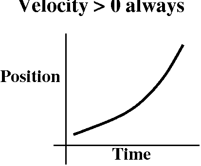 If velocity is always
positive, then position is moving steadily right.
Another way of thinking about this is graphical. If you wish, you
could imagine position as a function of time. Then the "progress" of
time might be the horizontal axis, and position in this diagram would
be the vertical axis. Position getting bigger would mean that the
graph of position versus time would be getting higher. So a
qualitative picture of this sort of graph is shown to the right.
Simple (?) observation #3
I will reverse the sign of the derivative. So here suppose f is
differentiable, and in some interval I we know for some reason that
f´ is always negative. What happens here? Well, take two
points, x1 and x2 in I with
x1<x2. MVT says that
(f(x2)–f(x1))/(x2–x1)=f´(c)
Now let's see: the right-hand side is now supposed to be negative. The
bottom of the left-hand side is positive (since
x1<x2 means
x2–x1>0). So we have a fraction with a
positive bottom equal to a negative number. So the top of the fraction
should be negative. That means f(x2)–f(x1)<0
so that f(x1)>f(x2). So what do we know:
IF f´ is negative,
THEN x1<x2 implies
f(x1)>f(x2).
Physical meaning
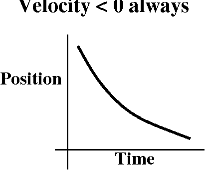 Again, derivative corresponds to velocity, and position corresponds to
the original function (and higher still means position is more to the
right, and lower position means more to the left on the line),
then:
If velocity is always
negative, then position is moving steadily leftt.
Again, we could think graphically. Position is a function of
time, the "progress" of time is the horizontal axis, and
position is the vertical axis. Position getting
smaller would mean that the graph of position versus time would be
getting lower. A qualitative picture of this sort of grpah is
shown to the right.
Further definitions
A function f is increasing on an interval I if whenever we take
x1 and x2 in I with
x1<x2, then
f(x1)<f(x2).
A function f is increasing on an interval I if whenever we take
x1 and x2 in I with
x1<x2, then
f(x1)<f(x2).
Facts
MVT implies:
If f´ is positive on an interval, then f
is increasing on that interval.
If f´ is negative on an interval, then f
is decreasing on that interval.
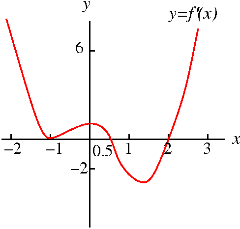 What we can say with graphical (qualitative) evidence
This is basically a discussion of problem 24 in section 4.3. The
problem gives a graph of the derivative f´(x) of
a function f(x). Please let me repeat: the graph is the
derivative of the function. I've attempted to copy the graph in the
picture to the right.
First, we are asked to "find the critical points of f". Since f is
differentiable (otherwise we wouldn't be looked at a graph of f´,
darn it!) the critical points here are where f´(x)=0. Look at the
graph. The curve crosses the x-axis at three values of x: –1, 0.5, and
2. These are the critical points of f.
Then we are asked to determine whether these critical points are local
max or local min or neither. So let me think through this with you.
|
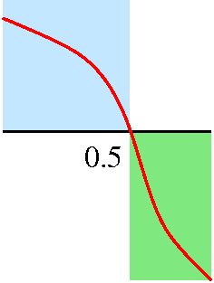
Local analysis near x=0.5
Look closely at the graph of f´ in a small interval to the left
of x=0.5. The graph (inside the very light blue region) is above the
x-axis. So in this interval, the derivative is positive and
therefore the function is increasing. Look now at the graph of
f´: in a small interval to the right of x=0.5. The graph (inside
the very light green region) is below the x-axis. So in this interval,
the derivative is negative and the function is
decreasing.
|  |
What should the graph of f (not the derivative!) look like? To
the left of 0.5, the function is increasing. The derivative at 0.5 is
0, so the tangent line is horizontal. To the right of 0.5, the
function is decreasing. Surely f has a local maximum at 0.5. I can't
tell the value of f(0.5), but I can tell you that value is
larger than f(x) for nearby x's, on either side of 0.5
f has a local maximum at 0.5.
| 
|
|
Local analysis near x=2
The situation is similar but reversed near x=2.
A "blow up" of the graph of f´ near x=2 is shown to the right.
In a small interval to the left of x=2, the graph of the derivative
(inside the very light blue region) is below the x-axis. So in this
interval, the derivative is negative and therefore the function
is decreasing. The graph of f´: in a small
interval to the right of x=2 is inside the very light green
region, above the x-axis. So in this interval, the derivative is
positive and the function is
increasing.
|  |
What should the graph of f (again, the graph of f, not of its
derivative!) look like? To the left of 2, the function is
decreasing. The derivative at 2 is 0, so the tangent line is
horizontal. To the right of 2, the function is increasing. Surely f
has a local maximum at 2. Again, we don't know the actual value of
f(2), but we do know its relative value. f(2) is
smaller than f(x) for nearby x's, on either side of 2.
f has a local minimum at 2.
| 
|
|
Local analysis near x=–1
I saved the most interesting (or maybe most irritating!) for
last. What do we see when we look very closely at the derivative near
x=–1? Well, to the left of –1 the derivative is positive,
above the x-axis, so the function itself should be increasing
in that interval. And to
the right of –1, the derivative is also positive, so the
function is also increasing there. That's what the graph of the
derivative of f declares.
|  |
The graph of f will show some delicate (?) behavior near –1. In a
small interval to the left of –1, we know f should be increasing (as
we walk from left to right, the graph will go up). And the same sort
of qualitative behavior will be true for the graph of f in a small
interval to the right of –1: up again. In fact, the graph is just
going up, increasing in the whole interval. The most fascinating (?)
aspect is that since f´(–1)=0, we'd better draw the graph of f so
that it has
a horizontal tangent line at –1. And that's what I've tried to show to
the right. If you are not used to this sort of kink in a graph, take a
look.
f has neither a local minimum nor a local maximum at
x=–1.
| 
|
| |
An office hour question
Mr. Orrico asked me in my office before
class about problem 28 of section 4.3. Here y=x(x+1)3 and
you are asked to find the critical points and find intervals in which
the function is increasing and decreasing. He found y&3180; and found
that it was equal to 0 at exactly two values of x, –1 and
–1/4. So the derivative is not zero in the interval
(–∞,–1) and in the interval (–1,–1/4) and in the interval
(–1/4,∞).
How many SIGNS can the derivative have in the interval (–1/4,∞)?
Well, I think the derivative, which is a polynomial, is continuous. If
it is both positive and negative in that interval then the
Intermediate Value Theorem tells me that the derivative must be 0
inside the interval. But it is not zero. Therefore the
derivative can have only one sign inside (–1/4,∞). Similar logic
tells me the derivative can have only one sign in the the interval
(–1,–1/4) and only one sign in the interval (–∞,–1). I don't
know what the signs are, but I do know that the sign doesn't
change. How can I discover what the sign is in the interval
(–1/4,∞)? I can check one value of f´ inside that
interval. Any value will work, and I should just choose something
that I find simple to compute with. I could choose 37 or
1,028,405.008. Or just 0. In fact, I don't even need to compute too
well -- I just need enough information to check what the sign is. So
that logic makes the problem easier.
|
| |

Maybe you'll believe this one ...
Here is a machine-generated graph of f(x)=x3 for x "near" 0
(well, for x between –1.1 and 1.1). Look closely at it. The local
behavior is very much like the local behavior of the text example near
–1.
The derivative is 3x2. This is positive if x is not
0, so certainly the function is increasing for x<0 and is
increasing for x>0. We paste these pieces together, and I think
that f is increasing for all numbers. There are several things to
notice "at 0" (actually, both at 0 and near 0). The tangent line is
horizontal. The curvature (!!) changes. The curve to the left of 0 is
concave down and, to the right of 0, it is concave up. I
will spend more time on such phenomena during the next lecture.
The First Derivative Test
Here is how, maybe, you could detect whether a critical point is a
local minimum or a local maximum or neither.
| Suppose f
has one critical point in an interval. |
|---|
| IF | THEN |
|---|
| f´>0 to the left of the c.p. |
f´<0 to the right of the c.p. |
| The c.p. is a local max. |  |
|
| f´<0 to the left of the c.p. |
f´>0 to the right of the c.p. |
| The c.p. is a local min. |  |
|
| f´ has any other sign assortment (positive/positive or negative/negative) |
The c.p. is neither. It is not a
local max and not a local min.
|
Actually I think about the local pictures and don't memorize the
algebra (with only 4 brain cells, for every fact I learn, it seems
that I must forget
two). I hope that you can see that appropriate local pictures for the
last line are (positive/positive)  and (negative/negative
  . You may prefer to think about the algebraic versions, but
the key idea is that the sign of the first derivative on both sides of
the critical point provides enough information to decide local max/min
questions.
A simple algebraic example
Here is problem 33 of section 4.3. The general instructions are to
find critical points and the intervals where the function is
increasing and decreasing, and then apply the First Derivative Test to
each critical point. Here f(x)=x4+x3.
Certainly f´(x)=4x3+3x2 and we set this
equal to 0, factoring: x2(4x+3)=0. The roots are 0 and
–3/4. These are the only places where f´ is 0. Notice that
f´ is continuous. This means if we test the sign of
f´ "between" the critical points, then we know the sign in each
of the intervals whose boundary is a critical point. This is because
if the sign changes, then (continuity, Intermediate Value Theorem)
there would have be a place where f´ is 0. This is a very
useful observation if you want to be lazy and efficient.
Testing the signs
We need to look "between" (on both sides of!) 0 and –3/4. Well, I bet
that f´(10)=4·103+3·102 is
positive. I bet also that
f´(–10)=–4·103+3·102 is
negative (thousands are way bigger than hundreds, and the parity
[even/oddness] of the powers makes this easy. What about really
between 0 and –3/4? I think in class we looked at x=–1/2. Then
f´(–1/2)=4(–1/2)3+3(–1/2)2=(–1/2)+(3/4) is
positive. So now in my head I have a picture of the real line:

What's important here is not the specific example but the
process. With a very small amount of work (compute derivative, find
critical points, take a few carefully chosen values of the derivative)
I can conclude:
- f is decreasing in the interval (–∞,–3/4].
- f is increasing in the interval [–3/4,0].
- f is increasing in the interval [0,∞).
- f has a local minimum at x=–3/4.
- f has neither a local minimum nor a local maximum at x=0.

Actually, f is increasing in the whole interval [–3/4,∞). The
type of each critical point is clear by using the First Derivative Test.
If you don't believe me, then take a look at a computer-generated
graph of y=x4+x3 to the right. Here, I will make
a bold statement: if I've done my critical point analysis correctly, I
think I would believe more in what it told me than in a
computer-generated graph. Formulas that make deceptive graphs are known.
|
My friend Francine drives again ...
 I don't want to get into legal trouble. The "logo" of the (beloved!)
New Jersey Turnpike is shown to the right. I am using it here totally
for educational purposes. Sigh. Only education. Really. No DVD's, no
music videos, no Latin American film rights, no web things. Really,
really.
After this assurance from the cowardly and worried writer, I remind
you that a previous drive of Francine on the Garden State
Parkway had been analyzed earlier
using the Intermediate Value Theorem.
The turnpike has a restricted number of entrances
and exits. Suppose Francine
- enters the turnpike at Interchange 4
("NJ73, Camden, Philadelphia"), Milepost 34.5, driving north at 8
AM.
She does not want to miss her calculus lecture, and therefore
after a rapid drive north, - exits the turnpike at Interchange 9 ("NJ-18,
New Brunswick"), Milepost 83.3, at 8:40 AM.
She should recieve a speeding ticket using
the following analysis.
Let's model the situation the following way. Suppose f(t) describes
Francine's position in miles on the turnpike, and t is the time, in
hours, after 8 AM. Then what we know is the following:
f(0)=34.5 and f(2/3)=83.3 (40 minutes is
two-thirds of an hour).
Then MVT asserts there is some time c
between 8 AM and 8:40 AM so that
f´(c)=(83.3–34.5)/(2/3–0)=48.8/(2/3)≈73.207. Since the speed limit on
that portion of the turnpike is 65 MPH, MVT shows that Francine was
speeding.
The Intermediate Value Theorem provides some information about
Francine's driving. It tells us that she passes through every place
(position) on the highway between Milepost 34.5 and Milepost 83.3 at
some time between 8 AM and 8:40 AM. This is somewhat indefinite.
The Mean Value Theorem gives more quantitative information,
also in a rather indefinite style (heck, we're given only outline
information!). It declares that the velocity (the derivative) must be
exactly 73.207 at some time between 8 AM and 8:40 AM.
The chunks of information have different flavors but mostly I think
that MVT information has more uses.
Semester project, honors course
Why doesn't the state actually use the information it has for such
things? It does have entrance/exit times and specifications of which
interchanges occur, etc. Explain in detail, with citations of specific
laws. Sigh. |
Quantitative information from the derivative
Here is a Math
Problem. Suppose you know the following about a
differentiable function:
f(5)=7 and, for all x, f´'s values are
between 40 and 60
(that is, 40≤f´(x)≤60).
What can you say about f(10)?
This seems to be very abstract and very silly. Let me translate it
into physical language, however.
A Physical Representation of the Math Problem:
Suppose f(t) represents the miles that have been traveled down a road
at time t (in hours, I guess AM!).
At 5 AM, you are 7 miles does the road.
Your speed is always between 40 and 60 mph.
What can be said about your position at 10 AM?
Somehow, phrased this way, the problem seems much more easily handled,
even to me, with a brain accustomed to math stuff. "Golly," I
might say, "In 5 hours you drive at least 200 [that's
5·40] miles and at most 300 [that's 5·60]
miles, so your position is between 207 and 307 miles down the
road."
We are actually using MVT reasoning on this. Look:
By MVT, [f(10)–f(5)]/[10–5]=f´(c), for
some c between 5 and 10.
But the derivative is between 40 and 60, and f(5)=7.
So 40≤[f(10)–7]/[5]≤60
Multiply by 5 and then add 7.
And 207≤f(10)<307.
The advantage of the mathematical approach is that it will apply to
all situations where we have a model and some estimate of the
derivative and knowledge of the function at one value. We then can
"predict" some estimate of the function at another value.
And even more (a possible QotD!)
Here is
what would have been the QotD, with my apology because I ran
out of time.
Suppose you know that f(0)=7 and
f´(x)=sqrt(1+x3). What can you tell me about f(2)?
MVT says that f´(c)=[f(2)–f(0)]/[2–0]=[f(2)–7]/2. Since
f´(c)=sqrt(1+c3) and c is between 0 and 2, I
bet that
1≤f´(c)≤3. Why is this? Well, f´ is increasing (you
can take the derivative and the derivative is always positive in that
interval so the function is increasing) and thus
1=sqrt(1+03)=f´(0)≤f´(c)<f´(2)=sqrt(1+23)=3.
Therefore 1≤[f(2)–7]/2≤3. Multiply by 2 and add 7. The result is
9≤f(2)≤13.
Thursday,
October 22 (Lecture #15)
We begin today the last half of the course.
Special added attraction (I hope)
I have been getting "customers" at my Tuesday office hour and I
would like to encourage this. So I will enlarge the office
hour (?): it will run from 11 AM to 1 PM. Part of my job, which I do
happily, is to help you learn and office hours can be useful. I
do remark, though, if you haven't visited, that my policy is to sit in
my chair, sluglike, and have students write things on the
board. You do the work. And as I remarked in class, if I'm
asked a question, I will frequently respond by requesting that people
look in the textbook -- the text should be used. Otherwise it
is a rather expensive decorative item.
Today we discussed the material in section 4.2, which is very
important, perhaps the core of most applications of mathematics in
engineering and applied science. Section 4.2 covers the ideas well,
and the class discussion (it was as close as we've gotten to a
discussion, at times) was an effort to familiarize people with the
ideas and methods which are quite important. I just wrote the boxed
items from section 4.2 on the board, and we went through them one by
one.
The difficulty now (from the instructor's point of view!) is
controlling the number and complexity of examples. There are many,
many, many interesting examples coming from real applications.
The class interaction was rapid, and maybe I spoke too fast at times
(I'm sorry). The examples below are generally similar to the ones
discussed in class.
Extreme values on an interval
I wrote the textbook's definitions of
Absolute minimum
and
Absolute maximum
on the board. I remarked that I
never understood definitions until I had examples that did and did
not satisfy the definitions. So I will assume that you have a
textbook next to you (I don't want to just copy what's there). You should know the definitions. The
situation the definition deals with is an interval, I, which is the
domain of the function, and a function, f, defined on that interval.
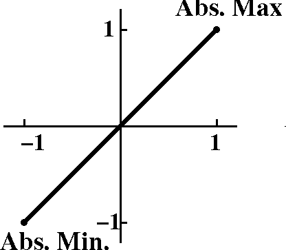
YES!
Here is an example of a function
and an interval, where there is both an absolute maximum and an
absolute minimum.
Here I=[0,1] and f(x)=x. Then f has an
absolute maximum at x=1, where f's value is 1, and f has an absolute
minimum at x=0, where f's value is 0.
another YES!
 Another example, where the interval is an open interval and the
function is still fairly familiar.
Suppose I=(Π/4,7Π/4) (this does not
include endpoints!) and f(x)=sin(x). This f has an absolute maximum at
x=Π/2 where f's value is 1. It has an absolute minimum at x=3Π/2,
where f's value is –1.
NO!
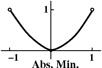 The first NO! example we had was rather subtle. I think it was
something like this.
The interval was (–1,1) (an open
interval, which does not contain its endpoints. The function was
something like f(x)=x2. There is an absolute minimum at
(0,0), but ... what would be "your" candidate for an absolute max? Any
number you choose which is close to 1 will have a number even closer
to 1 and bigger. For example, if you were to assert that f has an
absolute max at .99998, I would tell you that f's value at .9999999998
was bigger. If you said to me that .9999... (infinitely repeating) was
where an abs. max was located, I would reply that if you are
sophisticated enough with decimal notation to know about such things,
this indicates a certain geometric series whose sum is 1: the notation
.9999999.... is just another "address" for the number 1. And in this
case, the domain does not include 1 and does not include –1. So
this function in this domain does not have an absolute max.
NO!
 Another no example, which I think is fairly distressing, is gotten by
taking I=(0,1) (the open interval which does not have
endpoints) and the function f(x)=x. This is certainly a simple
function and a simple interval. This function on this interval has
no absolute max and no absolute min. I
think a person who is understanding this example for the first time is
really augmenting their intuition.
Why doesn't it have abs max or min? Well, certainly x=1 and x=–1
are not eligible locations for them, since both of these x's are
not in I. Now let's consider any other x in I. If we
microscopically (?) examine the local appearance of the graph of f(x)
near that x, it will always be a tilted line segment. To the left,
there are lower points on the graph, and to the right there are higher
points on the graph. That certainly implies our candidate is not
valid.
 Another NO!
Here is maybe a simpler example. Look at f(x)=tan(x) with the interval
(–Π/2,Π/2). I've only supplied a little doodle (?) of the
graph to the right.
Certainly there will be no absolute maximum and no
absolute minimum, since tan(x)→+∞ as
x→(Π/2)– and tan(x)→–∞ as
x→(–Π/2)+.

A more artificial NO!
Suppose the domain is [–1,1], which is a closed interval (includes its
end points) and which is bounded. Those two attributes (closed and
bounded) turn out to be important in the theory, as is described just
below. Now define f(x) piecewise: it is 0 when x=0 and it is 1/x when
x is not 0. Part of the graph of this function is shown to the
right. And if you think this is a silly example, I will totally
agree. But why is it silly, and what is there about it which is
not "nice"? Understanding one's feelings about such things is
sometimes very helpful. I don't like this example because the function
is quite clearly not continuous at 0 (the limit as x→0 of f(x)
does not exist). I also don't like this function because it certainly
does not have an absolute maximum and does not have an absolute
minimum.
Existence of extreme values on a closed and bounded interval
In many situations mathematical models are created which need maximum
and minimums. In business, we might be interested in lowest cost (min)
or highest profit (max). In more physical situations, many people want
lowest energy or least work. Or greatest volume or ... the
applications are numerous. Before searching for max or min, we might
want to know that such things exist (apparently they don't always --
look at the examples we have for NO!).
The following result can be proved, that is, deduced from
generally accepted and more obvious statements. The process of
deducing it is rather lengthy, and takes up a substantial amount of
Math 311. I request politely that you, as student engineers and
applied science types, be willing to accept the statement as
true. Most of the proofs of this statement do not supply any
method for actually getting the predicted max and min. So:
A theoretical result
Suppose I is a closed and bounded interval (so it is [a,b]), and
suppose that f is continuous. Then f has an absolute maximum and an
absolute minimum on I. So there are xM and xm in
I so that f(xm)≤f(x)≤f(xM) for all x's
in I.
This result does not tell how to find xM and
xm. It does not tell how many xM's and
xm's there may be (there may be many, but at least one of
each is guaranteed). For functions that are likely to be used
in practice, we will outline a useful strategy. First some more
definitions.
Local extreme values
f has a local maximum at x if f's value at x is the largest in
some open interval containing x. The most important and maybe
most confusing part of that sentence is "open interval". The dual
definition is: f has a local minimum at x if f's value at x is
the smallest in some open interval containing x.
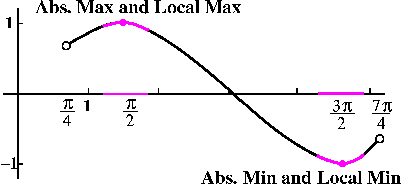
YES!
Here is a very simple example which is the same function and domain as
before. The absolute min is a local min. The absolute max is a local
max. I have put magenta in the
domain and on the graph to indicate the relevant open intervals.
A shocking NO!
 Again look at (0,1) and f(x)=x, choices which are very simple.
This function has no local min and no local max. Just as before, the
only points you might want to consider are the endpoints. But notice,
please, that the endpoints are no inside an open interval of
the domain. The right endpoint has no open side to the right, and the
left endpoint has no open side to the right. This example is really
quite annoying and unexpected if you're new to this game.
A zoo of YES and NO
Below is a collection of pictures. This probably is "Too much
information" but I tried to write all of the possibilities. It
wouldn't be difficult to write some fairly simple formulas whose
graphs qualitatively have the same behavior. I wanted to show that
"local" and "absolute" have no necessary logical relationships.

Critical points
These turn out to be very important. f has a critical point at
x if either f´(x)=0 or f´(x) does not exist.
The picture below is a zoo of critical points. Again, maybe this is
too much information. I do hope you get the feeling that local maxes
and local mins occur at critical points. This is true.

Geometrically, the derivative doesn't exist at the "point" of |x|
because the graph is not locally linear: no matter how much the graph
is magnified near (0,0), the result does not begin to resemble a
straight line. As for x1/3, this graph is the flip over the
main diagonal of x3. the x3 graph has a
horizontal tangent line at (0,0), and the geometrically valid tangent
line for x1/3 at (0,0) is certainly vertical. But the
derivative computes the slope of the tangent line, and vertical lines
have no slope. So there is no value for the derivative at x=0 (the
derivative formula is of course (1/3)x–2/3 and because of
the negative exponent 0 is not in the domain of f´(x) since we
are not allowed to divide by 0. The function x2/3 has
derivative (2/3)x–1/3 and this is certainly o.k. away from
0. But, again, the behavior near (0,0) isn't locally linear. The
"point" on this graph is sharper (!) than on the graph of |x|. It has
a name: it is called a cusp.
Fermat's theorem on local extreme values
If there is one single result which has kept math people prosperous
over the last three centuries, this is it.
If f is differentiable at x and if f has a local max or a local min at
x, then f´(x)=0.
 In this case I think it is useful for a practicing engineer to
have some feeling for why this result is correct. Look at the picture
to the right.
I drew what happens if you've got a local max. To get the local min
picture, just flip things over. What should you notice about this
picture? Well, the secant line from the left has a positive slope and
the secant line from the right has a negative slope. IF the derivative at the local max exists, it
will be the limit of things with different signs. The only way this
can occur is if the slope "at" the local max is 0.
Notice, though, that we need information from both sides. This
is why we are considering local maxes and
mins. If we don't have the two-sided information, we won't get the
disagreement of signs which compromises (?) at a zero derivative.
Extreme Values on a closed and bounded interval
Here I describe a procedure which provides a method for computing the
absolute max and absolute min of a function in an interval in many
cases, including almost all situations which arise in practice.
- Look at a continuous function on [a,b]. Theory says there's an
absolute max and an absolute min.
- Check the endpoints, a and b. The abs max and abs min could be there.
- If the abs max and abs min are inside then: either the function is
differentiable (and by Fermat the derivative is 0) or the function is
not differentiable. So find all the critical points inside the interval.
- Compare the values of f at the candidates you found: the endpoints
a and b and the critical points inside the interval.
Theory and practice
Mr. Theory asserts that
there must be absolute max and absolute min for functions and
intervals which satisfy the hypotheses of the theorem. But the theorem
doesn't give any advice about the location of these values. Indeed, if
you are naive, you might waste a huge amount of time just trying
random values of the function and trying find big and small
values.
Ms. Practice says to follow the
process above, and you've got to find the max and min. The advantage
is that in most "real" cases there are only a few critical points, and
the procedure allows you to narrow the search for abs max and min to
only a few numbers.
I will admit that in practice, though, it can be confusing. You look
at f(a) and f(b). You compute f´(x). Where is it 0? Where does it
not exist? Take those numbers and plug them back into f. So there are
two functions, f and f´, wandering around. You need to understand
what's necessary.
I concluded the lecture by solving a few of the many problems in
section 4.2. It can be argued that (as I said) these are toy
problems but you should get familiar with the method using these
toys, and then you can play (?) with more realistic examples.
Section 4.2, exercise #16
Find the extreme values of 2x3–9x2+12x on [0,3]
and [0,2].
I think I discussed [0,2] in class. Let me analyze [0,3] here. I will
try to be strict and not distract myself with pictures. I see my
initial task as creating a list of the possible locations of the
extreme values. Well, we will include the endpoints 0 and 3. Now we
need any critical points inside [0,3]. The derivative is
6x2–18x+12. The derivative formula for this nice
function, a polynomial, is valid everywhere. Let's see where it is
equal to 0. So:
6x2–18x+12=0 means
6(x2–3x+2)=0 means
6(x–2)(x–1)=0.
Please note that I sincerely doubt you will encounter very many
polynomials which can be factored in real applications. So the roots
are at 2 and 1.
The list of candidates is: 0 and 3 (endpoints) and 1 and 2 (critical
points). The values of the original function
2x3–9x2+12x at these points are: 0 (at
x=0), 9 (at x=3), 5 (at x=1), and 4 (at x=2). The absolute max is 9
and the absolute min is 0 on the interval [0,3].
I don't need to examine any other values. We're done.
Section 4.2, exercise #38
We should look at y=(1–x)/(x2+3x) on the interval
[1,4]. The only initial worry is whether this formula defines a
continuous function on the interval, but all of the input x's are
positive, and I am sure that the bottom, x2+3x, won't be 0
for positive x's.
My candidate list includes the endpoints 1 and 4. We need dy/dx. This
is (Quotient Rule)
(–1)(x2+3x)–(1–x)(2x+3)
------------------------
     (x2+3x)2
Where is this equal to 0? The only
way a fraction can be 0 is if the TOP is 0 so forget
about the BOTTOM! We solve (–1)(x2+3x)–(1–x)(2x+3)=0.
(–1)(x2+3x)–(1–x)(2x+3)=0
means –x2–3x+(x–1)(2x+3)=0 means
–x2–3x+2x2+x+3=0 means
x2–2x+3=0 means (x–3)(x+1)=0.
Again, this is not "real". Real polynomials rarely have nice roots,
and almost always the roots can only be found approximately. Well, the
TOP=0 when x=3 or x=–1. We discard x=–1 because it is not in
the interval of interest, [1,4]. We only need critical points inside
the interval.
Our list of candidates in this case is composed of the endpoints
1 and 4 and the critical point 3.
The values of the original function (1–x)/(x2+3x) are:
0 (at x=1), –3/28 (at x=4), and –2/18 (at x=3). The absolute max is at
0 (that's easy). Then (if I'm doing this "by hand") I need to worry a
bit about which of the other two values is more negative. In fact,
–2/18=–1/9 is less than –3/28 (because that is larger than –3/27 -- or
just compute them). So the absolute min is –1/9.
Again, the whole idea is that we really don't need to check many
values of the function. This turns out to be terrific. BUT in order to do this successfully, even with
toy problems, and to do things which occur later, every day in
this course, you will need to be able to compute the derivatives of
functions defined by formulas. Please know how to do this.
| Tuesday,
October 20 | (Lecture #14) |
|---|
Two very useful tricks
The lecture today will discuss two extremely useful "tricks" which are
constantly used, both computationally and theoretically. The relevant
textbook sections are 4.1 and 4.8. Please do not get distressed
at the numbering of the sections. The two techniques are quite related
-- they use the basic idea that a tangent line is close to the curve.
Some numerical evidence
I began by presenting some numerical "evidence". Here is a table of
numbers and their square roots which was examined by students. The
table has 20 digit accuracy, far more than any real world application
I know of. But the point of what's given here is to help people think
about things. The table
has a few more entries than I wrote on the board, and since I got it
straight from the computer, it has all 20 digits.
| Number | 20 digit square root of the number |
|---|
| 4. |
2.00000 00000 00000 0000 |
| 4.1 |
2.02484 56731 31658 6933 |
| 4.01 | 2.00249 84394 50078 5728 |
| 4.001 |
2.00024 99843 76952 8199
|
| 4.0001 |
2.00002 49998 43751 9531 |
| 4.00001 |
2.00000 24999 98437 5020 |
| 4.000001 |
2.00000 02499 99984 3750 |
| 4.0000001 |
2.00000 00249 99999 8438 |
I wanted people to examine the table for patterns. The first column
was, of course, 4{period}{some 0's}1. The second column, well, since
the square root of 4 is 2, and the numbers in the first column were
close to 4, then since square root is a continuous function, the
numbers in the second column were close to 2. But what's the pattern
of closeness? There are more 0's between the 2 and the first non-zero
digit. But the non-zero digits seem to have some pattern. For example,
consider the entry corresponding to 4.0001. That entry is 2.000024999
8437519531. There are 4 zeros between "." and "2". But the structure
of the non-zero digit string following is 24999998 and it sure looks
like it wants to be a bit simpler, just 25000000. What's going
on?
The algebraic way
Well, we have written the following a large number of times.
f(x+h)=f(x)+f´(x)h+Err(h)
and we know that the Err(h) term should →0 faster than a
multiple of h. In the case we have above, f(x)=sqrt(x) and we're
considering things that happen what x=4. Well,
f´(x)=(1/2)1/sqrt(x). At x=4, we get f(4)=2 and f´(2)=1/4
and this is .25 decimally. So the equation becomes
sqrt(4+h)=2+(.25)h+Err(h)
(Here the Err(h) term was also called H.O.T., for "higher order terms"
earlier in the course.
If we just want an approximation, hey, we could forget the Err(h) term
and get
sqrt(4+h)≈2+(.25)h
Here I am using the weird symbol ≈ for the phrase "approximately
equal" and I am deliberately not being too precise, right now,
about what this means. But let me rewrite the table above, now with
more decorations (!).
| Number | 20 digit square root of the number |
|---|
| 4. |
2.00000 00000 00000 0000 |
| 4.1 |
2.02484 56731 31658 6933 |
| 4.01 | 2.00249 84394 50078 5728 |
| 4.001 |
2.00024 99843 76952 8199
|
| 4.0001 |
2.00002 49998 43751 9531 |
| 4.00001 |
2.00000 24999 98437 5020 |
| 4.000001 |
2.00000 02499 99984 3750 |
| 4.0000001 |
2.00000 00249 99999 8438 |
Here what is underlined is essentially the 2+(.25)h stuff. Look: the
Err(h) term is shrinking twice as fast as the h is shrinking. And it
is negative. So for 4.0000001, with 6 zeros, the 2+(.25)h with
h=.0000001 appears in 16 places (except you need to think a bit since
the correction is negative, and therefore it appears as a digit string
of 24 followed by 9's). So there is evidence (yes, I admit it, this
is a "toy" problem, and all the numbers are very easy!) that the
Err(h) is sort of h2.
 Geometric interpretation
What does 2+(.25)h mean? Look at the picture. Everything is not meant
to be totally, literally accurate, but I'd like the ideas to be
correct. The circular area on the graph is magnified. We have a point
(x,f(x)) on the graph. x is moved (I drew the picture so that h is a
small positive number, and x+h is to the right of x). In the local,
magnified picture, there's a right triangle. One leg, the "adjacent",
has length h. The other is labeled ?. The line is tangent to the graph
at (x,f(x)). But the slope of that tangent line is f´(x). The
slope of the line is the tangent of the angle that line makes with
respect to a horizontal line, such as the leg labeled h. So f´(x)
is the quotient of ? and h: f´(x)=?/h. And ? must be f´(x)h,
and this length is added on to the vertical height that (x,f(x)) has
from the x-axis. The result is f(x)+f´(x)h. Hey! Using the
tangent line to make that little approximation is exactly the
same as starting from (x,f(x)) and making the adjustment from x to x+h
by riding along the tangent line. This is why
f(x+h) f(x)+f´(x)h
is frequently called the tangent line approximation. It also
explains why, in our specific case, the approximation is always
greater than the true value, because the parabola on its side is
underneath the tangent line.
In class ...
I actually found the formula for the tangent line, y–2=(1/4)(x–4) and
then substituted in 4+h for x to get y–2=(1/4)h so that
y=2+(1/4)h on the tangent line. So the tangent line value is actually
this approximation. That's why it is called the tangent line or
linear approximation to f(x+h).
All together?
I would like you to see how all of these points of view actually
reinforce each other. As I've remarked in class, I like the pictures,
but I know that many people prefer a formula, and certainly still
others like to see convincing numbers. That's why I've tried to show
you these varied approaches.
What about the error?
What the heck is the error like? Is it big or small? What can
we say? Well, I first remarked that we could see in our specific case
that as we go from left to right on the graph, the tangent lines got
flatter (that is, the slopes of the tangent lines themselves
decreased). Each tangent line was on top of the curve. The
linear approximation was an overestimate, and (as we will see
later) since f´ is decreasing, the second derivative,
f&180;´, is negative. The sign of the error is more or less
determined by the sign of the second derivative. The linear
approximation is larger than the true value when f´´(x)<0
and it is smaller when f´´(x)>0. I didn't say anything
about the size (the magnitude) of the Error.
Irving
 Irving is someone who remembers a formula and tries to fit every
situation to a formula. So Irving remembers
f(x+h)≈f(x)+f´(x)h and something about sqrt(4)=2. He
decides to approximate sqrt(100) in the following manner:
f(x+h)≈f(x)+f´(x)h
becomes
sqrt(100)=sqrt(4+96)≈sqrt(4)+(1/4)(96)=26.
Here Irving uses f(4)=4 and f´(4)=1/4 and h=96. I don't think
that 26 is a very good approximation to sqrt(100)=10. Irving may
remember the formula, but I think the formula has been used
inappropriately.
It turns out that the magnitude or size of the Error is roughly
proportional to h2. When h is teensy-weensy (maybe that
word is too technical?) then h2 is much teensier than
h. This is what was shown above in the table. That we only get a
discrepancy of 16 (from 10 to 26) in this case is not as bad as it
could be. I am joking here, but the decision about when to use (and
"trust"!) the linear approximation may not be too easy in practice (as
Ms. O'Sullivan managed to get me to
admit!).
Fifth roots
Here is another "classroom" example of this approximation.
I know
that 321/5 is 2. What is a (useful) approximation to
(32+h)1/5? Here f(x)=x1/5 and
f´(x)=(1/5)x–4/5. So the formula
f(x+h)≈f(x)+f´(x)h with x=32 becomes
(32+h)1/5≈321/5+(1/5)(32)–4/5h
and (after arithmetic, since 32–4/5 is 1/16) this is
(32+h)1/5≈2+(1/80)h.
For example, 311/5 is reported as 1.987340 by a computer,
and the approximation (with h=–1) is
311/5=(32–1)1/5≈2+(1/80)(–1)=1.9875000. I didn't expect that the
approximation would be this good. Notice that
f´´(x)=(1/5)(–4/5)x–9/5 so
f´´(32)=(1/5)(–4/5)32–9/5 is negative. So just as
in the square root example, the estimate is larger -- an overestimate.
A more real problem...
One of the early experiments attributed to Galileo is observation of a
pendulum. He asserted that the period of a pendulum depended on the
length of the pendulum and was independent of the size of the angular
oscillation. This is really remarkable and means that maybe you can
use a pendulum clock to time things accurately --- only the length of
the pendulum matters and not how far or wide it swings. It turns out
this assertion is actually true only for small oscillations. Galileo
supposedly only observed small oscillations. A mathematical model of
pendulum motion (go to your physics instructor!) gives
d2θ/dt2 =(Constant)sin(θ) (here θ is the angle
between the pendulum and the vertical direction). This differential
equation is
too darn hard to "solve" (you will see why later) and so people
want a simpler model. If θ is
very small, then (since sin(0)=0 and sin´(0)=cos(0)=1) we can
substitute θ for sin(θ) and the equation becomes
d2θ/dt2 =(Constant)θ. This equation is much simpler
(I'll actually be able to tell you all about it in a few weeks). And
the predicted independence of period turns out to be true, with this
small oscillation assumption.
|
What is the square root of 4? Or the square root of 2?
Sigh. I'm fairly sure that the square root of 4 is 2. I would like to
know the square root of 2. Generally, there are many occasions when we
would like to solve f(x)=0. This
turns out to be impossible in terms of standard functions and
formulas even for relatively simple f(x)'s. Really what I wanted to
discuss was the single most widely used method of taking an
approximation to the root of an equation and improving the
approximation, that is, getting closer to the root. The improvement
technique is called Newton's Method. I called the old guess, G,
and the (hoped for) improved new guess, N.
 Newton's Method
Newton's method is a way to (try to) improve a guess at a root
of f(x)=0 when f is a differentiable function. The guess, G, is
(hopefully!) improved with the following process (as you read this,
please glance at the picture to the right). First, go up from G
until you "hit" the graph of y=f(x). The point will be (G,f(G)). Then
"slide down" the tangent line of the graph. The slope of that tangent
line must be f´(G) because it is tangent at (G,f(G)). The point
that this line hits the x-axis is the new guess, N. The picture is
rather simple and shows the new guess closer to a root of the
function. Again, this is a simple picture, and is the way we would
like the method to work. I will discuss more horrible
possibilities later, but right now I would like to get a formula for N
in terms of G. Well, the slope is f´(G), but this slope is also
equal to OPPOSITE over ADJACENT because the slope of a line is the
tangent of the angle that the line makes with the x-axis (this is the
same key idea we've already used once before in this lecture). Here
OPPOSITE is f(G) and ADJACENT is G–N. Therefore
f´(G)=f(G)/(G–N) which is the same as
G–N=f(G)/f´(G), so that
Newton's method
N=G–{f(G)/f´(G)}
|
|---|
For square roots
Suppose I want to compute or approximate sqrt(A). What I am describing
is the method that is actually used in most calculators and
computers. I need a function which has a root at sqrt(A). The simplest
candidate seems to be f(x)=x2–A and then
f´(x)=2x, so that G–{f(G)/f´(G)} becomes
G–{[G2–A]/2G} which is
{2G2–[G2–A]}/2G which is
[G2+A]/2G which is (1/2)[G+{A/G}]. That is, "Improve the
guess to a new guess, N, by taking the average of the old guess, G,
and A/G: N=(1/2)(G+[A/G])."
Here is the complete "coding" (writing and running of the "program")
for Newton's method to compute the square root of A=2 using Maple. Yes, this is silly, but you should see
again what the numbers look like.
> N:=G->(1/2)*(G+(2/G));
                                  N := G -> 1/2 G + 1/G
> N(2.);
                                       1.500000000
> N(%);
                                       1.416666667
> N(%);
                                       1.414215686
> N(%);
                                       1.414213562
> N(%);
                                       1.414213562
> sqrt(2.);
                                       1.414213562
The first command, N := G -> 1/2 G +
1/G defines how to replace the old guess, G, by a new
guess N. The symbol "%" means "Use the previous answer." If we
initially "guess" 2 as sqrt(2), then only 5 uses of Newton's Method
gets sqrt(2) to 10 decimal place accuracy.
 So just a few iterations (repetitions of N) makes the estimate close
enough to sqrt(2) that we can't tell the difference (to 10 decimal
digits)! This is pretty darn fast, and this is actually how your
calculator computes square roots. There is considerable evidence
suggesting that this method of computing approximations to square
roots has been known for 4,000 years. Try the key words Babylonian
square roots in a search engine. Human beings can be quite clever.
The picture to the right is an attempt to show you how Newton's method
works geometrically for the specific function f(x)=x2–4
with a specific initial guess of 3. So there's the graph,
y=x2–4, the parent parabola pushed down 4 units. Take the
initial guess at 3 (what's described now is all in magenta) and go up until you hit the
parabola. Slide down the tangent line until you hit the x-axis. Then
up to the parabola again, slide down the tangent line, etc. This is
very silly, but look at the magenta line segments. It is rather
difficult to draw them so that they can be seen, because they tend to
pile up so quickly at the point where the parabola and the x-axis
intersect. This is remarkably fast when it can be used, much faster
than bisection. Newton's method generally doubles (!) the
number of decimal digits of accuracy at each repetition. (This is
really really really good.)
Dividing is difficult
Of the arithmetic things we all learned early in grade school,
certainly division is the one that I and many other people believe is
the most difficult. To find, say, 1/7, you need to make some guesses
at places in the computation, and sometimes the guesses are just
wrong. Some "backtracking" is needed. What the heck can we do if we
want to tell machines how to compute this? Here, very briefly, is what
we can do.
Suppose A is a positive number and we want to compute an approximation
to 1/A. Well, 1/A is a root of f(x)=(1/x)–A. Then
f´(x)=–1/x2. Notice in all this, please, that
computing derivatives must be totally routine, or else everything
becomes much too hard. Then the Newton's method equation,
N=G–{f(G)/f´(G)} becomes
N=G–{[(1/G)–A]/[–1/G2]
and this can be simplified (changing compound fractions to simple
fractions):
N=G+[(G)–AG2]=2G–AG2
This means that to compute 1/7 we should do the following: replace an
old guess, G, by a new guess, 2G–7G2. Please
appreciate how easy this is compared to long division, with guessing
and subtracting and then doing it again! Here is what happens when we
try to use this: > INV:=x->2*x-7*x^2;
(Comment This defines how to replace the old guess.)
> INV(.1);
0.13
> INV(%);
0.141
> INV(%);
0.1417
> INV(%);
0.14284777
> INV(%);
0.1428571422421897
> INV(%);
0.14285714285714285450
This last answer is accurate to 17 decimal digits. This is almost
surely more than any moderately sane human being needs.
QotD
What is 101/3? More precisely, define a fairly simple
function f which has 101/3 as a root. Then use the initial
estimate of x=2 in Newton's method twice.
Here the function that I thought of is f(x)=x3–10. And
f´(x)=3x2. The Newton's method would take a guess, x,
and replace it by x–(x3–10)/(3x2).
If the initial guess is x=2, the replacement, which we hope is closer
to the true value, would be 2–(23–10)/(3[22]).
This is 2–(–2)/12=2+1/6=13/6.
Then replace 13/6 by {13/6}–({13/6}3–10)/(3{13/6}2)
The exact result is (not clearly!) 3277/1521 (yeah, I did
not do this by hand!).
How about decimal computation? If the initial guess is 2, then the
replacement is 2.1666666667 and that, in turn, becomes
2.1545036160. Sigh.
The computer reports that 101/3 is 2.1544346900 so that we
seem to have gotten about three decimal places of accuracy.
Three iterations gets 8 places of accuracy, and four iterations gets
15 places of accuracy. Is this exciting?
Bad things can happen
The Bisection Method is much slower than Newton's Method, but the
Bisection Method (assuming that the hypotheses are satisfied!)
always works. Newton's Method is notorious for fouling up,
sometimes especially when you don't want problems. Let me show you
what can happen.
Look at the picture to the right. It is a graph of a function,
y=f(x). The function has one root, at x=R. Let's examine the effect of
various initial guesses.

- If the initial guess is x=A, then bouncing up and sliding
down, etc., works really nicely. The repeats of Newton's Method
converge nicely and rapidly to the root, R.
- Suppose the initial guess is at x=B. Then up to y=f(x), and the
tangent line pushes the next guess way to the left. One should have (I
certainly don't have!) any feeling about what would happen out
there. Certainly things may not come back to the root.
- Suppose the initial guess is at x=C. Then Newton's Method pushes
the following guesses out and out and out to the right (think of a
curve that's asymptotic to the x-axis but has no root to the
right). So again the situation is highly unsatisfactory.
In practice people may check to see if things are working
well. Usually (experience!) it is when you don't check that
Newton's Method misbehaves.
|
| Thursday,
October 15 | (Lecture #13) |
|---|
How a rectangle changes
A rectangle is changing with time. At a certain time, its length is 7
inches, and is decreasing at .6 inches per second. At the same time,
its width is 3 inches, and is increasing at .5 inches per second.
Question 1 At that time, is the area of
the rectangle increasing or decreasing? At what rate is the area
changing?
Question 2 At that time, is the length
of the diagonal of the rectangle increasing or decreasing? At what
rate is the diagonal changing?
What I might think about this
Here is how I might think about this problem. I don't know how many of
these details I would write as I analyze the problem, but almost
surely I would think what I write here.
- The nouns of interest are rectangle, length, width, area, and
diagonal.
- I'd
probably make a sketch of as much of the situation as possible. The
sketch might look something like what it shown to the right.
 I would
label the sketch with as many of the "nouns of interest" (?) as
possible. I usually try to choose labels that sort of match the nouns
or ideas they designate (so I use L for length). I also try to
make the sketch match as much additional information as possible in
the problem. For example, I labeled the longer side of the rectangle L
mostly because in the problem statement, L was 7 at the "certain
time", while W, the width, was 3, and 3 is less than 7. There are two
diagonals in the rectangle, and the diagonals have equal length. The
diagonal I chose to draw and label with D is that one which completes
a right triangle with legs L and W, and the reason I chose that
diagonal is I was thinking ahead to the next step.
I am not trying to be silly about this problem. But, as much as
possible, I am trying to slow down and give a precise, step-by-step,
discussion of my approach to this problem.
- I would try to connect the variables algebraically, somehow making
the picture into equations. For example, I'll call the area, A, and,
although A is not shown in the picture, I do know that
A=L·W. Also, since I "completed" a right triangle with D as
hypotenuse, then the Theorem of Pythagoras tells me that
D=sqrt(W2+L2).
- Now what? Maybe I can
Answer the first question Since A=L·W, and we need to
know about dA/dt, I can try to d/dt the equation. I assume in
everything that I'm doing that I can differentiate things. So the
Product Rule gives us (since both L and W are functions of time) that
dA/dt=(dW/dt)L+W(dL/dt). At the "certain time" we know the values of
the four terms which appear on the right-hand side of the
equation. dW/dt is .5 (I'm not worrying about the units right now) and
W is 3. L is 7 and dL/dt is –.5 (here the interesting thing is the
–, and we need the minus sign because of the word
decreasing in the problem statement). Therefore
dA/dt=(.5)(7)+(3)(–.5)=3.5–1.5=2. The area of the rectangle is
increasing at the rate of 2 square inches per second.
- And I can
Answer the second question Here
D=sqrt(W2+L2), and we must d/dt this equation
also. Some care is needed. Again W and L are functions which vary with
time, that D's relationship with them is complicated. Use the Chain
Rule with some care. The result seems to be:
dD/dt=(1/2)(W2+D2)–1/2(2W(dW/dt)+2L(dL/dt)).
Now we "instantitate" with the values we have at the "certain time"
(but do it carefully!):
dD/dt=(1/2)(32+72)–½(2·3(.3)+2·7(–.6)).
Again, watch the darn signs. The result, if I do the arithmetic
correctly (!) will be dD/dt=(58)–½(–3.3). So the length
of the diagonal is decreasing (!) at the rate of
(58)–1/2(3.3) inches per second.
- Again, I will agree that this is not a profound
problem. But I'll also write what I stated in class: the
{in|de}creasing nature of the results sure isn't clear from the
problem statement (in fact, I had to arrange the numbers carefully to
get the qualitative differences: that the area is increasing
and the diagonal is decreasing: slightly weird).
As I mentioned in class, I am experienced but I generally need to read
this type of problem two or three times (at least) to make more likely
that I understand what is varying, and what information is given and
what information is requested. Even if the person who wrote the
problem is trying to be helpful, there can still be real difficulty in
comprehension.
How an annulus changes
An annulus or annular region is a region in the plane
which is between two circles which have the same center (concentric
circles). For example, you can see such a region if you drop a
rock into a quiet pond. There are likely to be a series of circular
ripples which spread radially and evenly from the point of impact of
the rock. Suppose we have an annular region changing with time. At a
certain time, the outer radius is 6 inches and decreasing at .3 inches
per second, and the inner radius is 4 inches and decreasing at .2
inches per second. At that time, is the area of the annulus increasing
or decreasing? What is the rate of change of the area?

This was the QotD.
Here's a discussion of a solution.
The geometry of this annulus is determined by the radii (that is the
plural of radius, I think). There is an inner, smaller radius which
I'll call r, and an outer, larger radius which I'll call R. The area
of the region is the difference of the area of the region bounded by the
outer circle, Π R2, and the area of the region bounded by
the inner circle, Π r2. The area, A, of the annulus,
is given by A=Π R2–Π r2. The extra
minus sign, together with the two uses of the word "decreasing" in the
problem description make the solution of the problem interesting to
me. I can't easily guess whether the area is increasing or
decreasing.
If we differentiate the equation carefully, the result is
dA/dt=2R(dR/dt)–2r(dr/dt). At the "certain time", we get
dA/dt=2·6(–.3)–2·4(–.2)=–3.6+1.6=–2 inches per
second. So the area of the annulus is decreasing at a rate of 2 inches
per second at that time.
An ant crawls on a parabola
An ant is crawling on the parabola y=x2. (Fairly absurd,
but maybe slightly more realistic and useful than the first two
problems.) Suppose that the horizontal, x, coordinate of the plane is
increasing at 6 units per second when the ant crawls through (?) the
point (2,4). How fast is the y coordinate of the ant's position
changing at that time?
So x and y are functions of time and y=x2. If we d/dt the
equation, the result is dy/dt=2x(dx/dt). When the ant is at (2,4),
this becomes dy/dt=2·2·6=24.
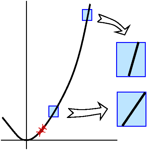 A bit more ant crawling
Suppose that the ant crawls on y=x2 so that the rate of
change of its first, x, coordinate is always 6 units per second. What
happens to the rate of change of the y coordinate as the x moves far
to the right? I'll try to both compute this and explain it.
Let's "think" about the situation. The picture to the right is to help
with thinking. If we take a tiny piece of the parabola, and blow it
up, the piece becomes almost a straight line (the parabola is
locally linear). For a piece near (2,4), say (similar to the
lower piece shown), the line is not too steep. For a piece "far" to
the right (as the upper piece shown), the line is rather
steep. Imagine the ant traveling in such a manner that the x
coordinate changes steadily with a rate of 6 units per second. There
will be different y changes to allow the ant to stay on the curve. In
the more right, more up box, the y change will be larger than the y
change needed in the lower box. So I conclude that dy/dt will grow as
the ant moves more to the right.
Now let's look at the algebra. y=x2 again implies
dy/dt=2x(dx/dt) and if dx/dt is always 6, then dy/dt=12x. Indeed, when
x→∞, dy/dt→∞.
Change the crawling
What if the ant crawls so that the vertical, y, coordinate changes
steadily at 6 units per second. Again the motion of the ant along
y=x2 moves to the right and up. What happens to the
x-coordinate change as the ant moves steadily up?
It might be useful for you to again consider the local linearization
pictures, which I hope will tell you in this case that if dy/dt is
constant, dx/dt must get smaller as the ant moves to the right. And
the algebra: since dy/dt=2x(dx/dt) and here dy/dt is supposed to be 6
always, we see that dx/dt=3/x. As x→∞, dx/dt→0.
Of course what I am doing is considering the velocity vector of
the ant's motion under various hypotheses concerning components of the
vector. This velocity vector is tangent to the ant's path, and this
geometric fact forces the other conclusions
A conical reservoir is being filled
A right circular cone is an object which shows circular slices
when cut by a plane perpendicular to its axis of symmetry. The sides
of the cones are formed by straight lines through the vertex. The
vertex of the cone is the pointy part.
Now suppose we have a reservoir which is a right circular cone with
its vertex at the bottom. The height of the cone is 30 feet, and the
base radius is 5 feet. The cone is being steadily filled by a fluid at
the rate of .2 cubic feet per minute. How fast is the depth of the
fluid changing when the fluid is 20 feet deep in the reservoir?
Oh mechanical engineers: "A fluid is defined as a substance that
continually deforms (flows) under an applied shear stress regardless
of the magnitude of the applied stress." I asked for some suggested
fluids and got almost no answers. Sigh.

The pictures show a right circular cone with vertex at the bottom. The
oblique view is prettier, I think, but a transverse "section" through
the axis is probably better for analyzing this problem. A formula
which certainly is needed follows: V=(Π/3)R2H is the
volume of a right circular cone with height H and base radius R. If
the fluid level is H and the radius of the fluid-filled volume is R,
then the volume filled by the fluid is V=(Π/3)R2H. We know
also that dV/dt=.2 (positive: the cone is being filled). Well, V seems
to have too many letters for this course (in calc 3, functions
involving several variables are dealt with). But there is a
geometrically forced relationship between R and H which I hope you
see. Look at the transverse picture and at several similar
right triangles. Ratios of corresponding sides must be equal for the
two right triangles shown, so 30/H=5/R and R=H/6 (I want V in terms of
H because the problem statement asks for the rate of change of the
depth of the fluid, which I believe is dH/dt). Therefore
V=(Π/3)R2H=(Π/3)(H/6)2H=(Π/108)H3. If
we d/dt the equation V=(Π/108)H3 being careful to use the
Chain Rule appropriately, the result is
dV/dt=(Π/108)(3H2)(dH/dt)=(Π/36)H2(dH/dt). Now
plug in the known dV/dt and the depth, H=20, to get
.2=(Π/36)(20)2(dH/dt). Therefore the rate of change of the
depth when the depth is 20 feet is .2/[(Π/36)(20)2]
feet per minute.
Please notice that since dV/dt is constant (.2) we know that
dH/dt=.2/[(Π/36)H2]. So we see that as H increases,
the rate of change of H decreases. This is because the
cross-sections of the cone's volume are steadily increasing so the
steady volume increase means that the height is not increasing as
much.
Another way (as done in class)
This isn't what I did in class. There I took the whole equation
V=(Π/3)R2H and d/dt'd it to get (Chain Rule and Product
Rule) dV/dt=(Π/3)2R(dR/dt)H+(Π/3)R2(dH/dt) . If H=30
and dV/dt=.2 we have
.2=(Π/3)2R(dR/dt)(30)+(Π/3)R2(dH/dt) but 6R=H
(deduced above and in class) implies first that when H is 20, R is
(20/6). Also it implies that 6(dR/dt)=dH/dt or dR/dt=(1/6)(dH/dt).
Then .2=(Π/3)2R(dR/dt)(30)+(Π/3)R2(dH/dt) changes to
.2=(Π/3)2(30/6)(21/6)(dH/dt)(30)+(Π/3)(20/6)2(dH/dt).
We can then solve the equation for the desired dH/dt. I think this
answer is the same as obtained by the earlier method.
| Tuesday,
October 13 | (Lecture #12) |
|---|
I think lecture #11 was the first exam. So here is (more or less) what
we did today.
Implicit differentiation can help find the derivatives of inverse
functions. The inverse function to sine was discussed yesterday by
Mr. Nakamura, but I will include a diary entry from a previous 151
course about this material.
arcsine
What's happening in the pictures below (left to right):
The first
picture is supposed to be a portion of the graph of sine. It is 2Π
periodic, and its range is [–1,1]. The green line is the "main
diagonal", y=x, which also happens to be tangent to y=sin(x) at
(0,0). This is because the slope of the tangent line is the derivative
of sine, which is cosine, and cos(0)=1. To get the inverse function,
we interchange inputs and outputs. Geometrically we flip the graph
over the mBBain diagonal, and get the second picture. The tangent line
is still tangent, but now, look at the red line. This demonstrates
that the flipped graph is not the graph of a function. It fails
the vertical line test to be a graph of a function. Thus we need to
cut away (!) part of the graph. The "clouds" in blue-green (?)
demonstrate what will be cut away. And what's left is shown in the
third picture. This is the official graph of y=arcsin(x): domain
[–1,1] and range [–Π/2,Π/2]. It has arcsin(0)=0, and the tangent
lines seem always to slope up, so the derivative should be
positive. And if we are very careful, the lines tangent to sine at
+/–Π/2 are horizontal, so the lines tangent to the flipped curve will
be vertical and have no slope so there will be no derivative at
+/–1. The derivative of arcsin should have domain (–1,1), the interval
without endpoints.

Consider this
process:
- y=arcsin(x) The inverse function
- sin(y)=sin(arcsin(x)) Using the inverseness
- sin(y)=x Recognition of inverseness
- cos(y)(dy/dx)=1 Implicit differentiation
- dy/dx=1/cos(y) Solving for
dy/dx
- Since sin(y)=x, x2+(cos(y))2=1, and so
cos(y)=+/–sqrt(1–x2). Which sign to take? In the
range we are considering between –Π/2 and Π/2, cosine is
positive. Also the slope of the tangent line is positive for
arcsine. We will take the + sign. And
cos(y)=sqrt(1–x2). Solving for dy/dx stuff in x
- So arcsin´(x)=1/sqrt(1–x2) Statement of
formula
We will go through this a few more times today. But in any case, the
derivative is 1/sqrt(1–x2). Notice that for –1<x<1,
this is positive, and that the derivative formula is not valid
at +/–1 as the geometric evidence predicts.
Example The derivative of arcsin(5x3–ex) is
[1/sqrt(5x3–ex)](5·3x2–ex)
using the chain rule.
|
arctan
What's the picture below supposed to show? The
initial picture is y=tan(x). This function is periodic with period Π,
and its domain does not include odd multiples of Π/2. The
function is rather simple looking (!), always tilted up, and has
vertical asymptotes at odd multiples of Π/2. Flipping to get an
attempted inverse function reveals lots of problems (I omitted the red
line here). The standard restriction is to throw out the "branches"
that don't intersect the horizontal axis, and that's what I've
attempted to suggest with the blue-green "clouds". Again, y=x is a
tangent line to both arctan and tan at (0,0) because the derivative of
tangent is (sec(x))2, and sec(0)=1/cos(0)=1. Arctan is very
useful. It "compresses" all of the real numbers into the interval from
–Π/2 to Π/2, so if you have lots of data and you don't know ahead of
time how big (+ or –) the data will be, composing it with arctan will
at least control it a bit. Now for the derivative. Notice that the
derivative of arctan should always be positive (the tangent lines all
tilt up) and that the slopes→0 as x→+∞ or as
x→–∞, since the arctan curve gets flatter there.

- y=arctan(x) The inverse function
- tan(y)=tan(arctan(x)) Using the inverseness
- tan(y)=x Recognition of inverseness
- (sec(y))2(dy/dx)=1 Implicit differentiation
- dy/dx=1/(sec(y))2 Solving for dy/dx
- Since tan(y)=x, x2+1=(sec(y))2 (much easier
than arcsine!). Solving for dy/dx stuff in x
- Thus arctan'(x)=1/(1+x2) Statement of
formula
The derivative function, 1/(1+x2), is always positive as we
thought. And as x→+∞ or as x→–∞, the function
1/(1+x2) does →0, so this formula does have the
desired behavior out towards the "edges".
Examples
I did several, maybe something like this.
The derivative of
arctan(e(5x4)) is
1/(1+(e(5x4))2·
e(5x4)·5·4x3: somewhat
of a mess, using the chain rule several times.
The derivative of arctan([x+1]/[x–1]) is
1/(1+{[x+1]/[x–1]}2)·{[1(x–1)–(x+1)1]/[(x–1)2]}
 Looking at a constantly accelerating rocket ship
Here is almost a real computation. It is my effort to show how arctan
can be used.
Let's consider a rocket ship launching vertically upward with constant
accelaration a. We know from physics class that at time t, the rocket
ship is {1/2}at2 high. Suppose we are standing a distance D
from the launch point of the rocket ship. The rocket ship starts from
velocity 0 and seems to move slowly. Then it seems to move
faster. Finally, when it is high up in the sky, its apparent motion is
slow again, although it is actually moving very fast. Let's call
θ the angle betwwen the ground and the rocket ship. How does
θ change with time? Well,
tan(θ)={1/2}at2/D={a/(2D)}t2 so that
θ=arctan({a/(2D)}t2).
The rate of change of θ with respect to time is dθ/dt,
which we could call angular velocity. What is it? The Chain
Rule tells us.
dθ/dt={1/(1+[{a/(2D)}t2]2)}{a/D)}t
I will act against many previous comments and simplify this, because I
will want to do further computations. So, after simplifying, we have
 dθ/dt={[(a/D)t]/(1+[{a/(2D)}t2]2)}={[(a/D)t]/(1+[{a2/(4D2)}t4])}.
The angular velocity begins small because the rocket ship is moving
very slowly. Later this gets larger as the rocket speeds up. But,
eventually, as the rocket gets very high in the sky, even though its
velocity might be quite large, the apparent position of the rocket
seems to change only slightly, so the angular velocity decreases
towards 0. The curve to the right describes this qualitative
behavior. If you consider the algebraic formula we just got for
dθ/dt you will see:
- If t is small, the bottom is 1+(Constant)t4, and
t4 is very small (small numbers get smaller even when
powers are done). So the bottom is ≈1. The top is
(Another constant)t, so we have that dθ/dt is about
(Another constant)t/1 so it must be small when t is small.
- If t is very large, then the top is t1 but the
bottom has t4 so certainly the bottom overpowers the
top. (Note: The word "overpower" is supposed to be sort of a joke
["powers of t" -- get it?] and I will show you later other ways to
decide that this formula for dθ/dt is small when t is large.)
So the formula and my understanding of the physical situation lead me
to realize that maybe there is some time, tMAX, where the
angular velocity is largest. What is that time? Well, it will occur
when the tangent line to the curve (the dθ/dt curve) is
horizontal. That means we need to find t so that the derivative
of dθ/dt is 0. So we need to consider what we could call angular
accelaration.
Let's differentiate
{[(a/D)t]/(1+[{a2/(4D2)}t4])}. we
need the quotient rule. Please realize that a and D are constants, and
t is the variable.
(a/D)(1+[{a2/(4D2)}t4])-[(a/D)t](0+{a2/(4D2)}(4t3)
-------------------------------------------------
              (1+[{a2/(4D2)}t4])2 .
This is (wonderful but traditional notation!)
d2θ/dt2. The wonderfully unsymmetric
placement of the 2's is done because ... because ... someone did it
centuries ago. Well, for which t is this 0? So we have a fraction,
TOP/BOTTOM. It will be 0 exactly when (and only when!) the TOP is
0. So we need to find t so that
(a/D)(1+[{a2/(4D2)}t4])–[(a/D)t](0+{a2/(4D2)}(4t3)=0.
This was confusing enough in class, and I can only hope that my messy
formulas can be understood here. Let's distribute. Some "miracles"
occur.
(a/D)+[{a3/(4D3)}t4]–{a3/(D3)}(t4)=0.
Now multiply by 4D3 (certainly this is not the only way of
making sense of this mess, but I like to get rid of fractions when
possible -- when you present this problem, go ahead and do the
algebra the way you like!).
4aD2+[a3t4]–{4a3(t4)=0.
The last two terms combine.
4aD2–3a3(t4)=0.
And now we "solve" for t by pushing the minus term to the other side
and dividing by some constants and taking the fourth roots (1/4):
So tMAX=((4/3)(D2/a2)1/4.
What a lot of work. You can now find the maximum angular velocity by
plugging in the expression for tMAX into the formula for
dθ/dt. The result is complicated and doesn't tell me much. There
is one thing which is somewhat amazing to me. Let me find the angle,
let me call it θMAX, at which the maximum angular
velocity occurs. So we need to plug tMAX into
θ=arctan({a/(2D)}t2). Here we go:
θMAX=arctan({a/(2D)}(tMAX)2)=arctan({a/(2D)}(((4/3)(D2/a2)1/4)
2)=arctan({a/(2D)}((4/3)(D2/a2)1/2).
Now look again at the input, the "argument", of arctan. The ((4/3)(D2/a2)1/2 stuff is really [2/sqrt(3)](D/a)
and this multiplies {a/(2D)} so lots of stuff cancels. Therefore
θMAX is arctan(1/sqrt(3)) which is Π/6 (o.k., darn
it, 30o) always. There is no a and there is no D in this
answer. I find this amazing and amusing (?). I wish that I understood
why this is true physically -- that is, if there were some
reasoning without all this algebra to convince me that the answer
should not have a and D. I don't know such reasoning.
Drop a rock (on any planet!)
Suppose you were at the top of a tall cliff on Planet X (for any value
of X!). And a distance D away on the horizontal top of the cliff an
alien dropped a rock. It would fall with some unknown acceleration due
to local gravity. If the cliff were tall enough (!!), as you looked at
it, the angle of inclination would increase. You would turn your head
faster and faster, until, exactly at angle -Π/6, the angular
velocity of the dropping rock would be a maximum. Then this angular
velocity (how fast you would be rotating your vision) would begin to
slow. WHY doesn't this depend on the
distance between you and the alien, and why doesn't it depend on the
local acceleration of gravity? I don't know (in some real
"physical" way) and I wish I did. If you have some insight, please
tell me. I thank you in advance.
|
arcexp (?)
Should this be called arcexp? Well, it isn't. The inverse
function to an exponential function is a logarithmic
function. This logarithm function is very important. The log
functions you may deal with include log10 (used in the
definition of pH, and for hand calculation in "the old days") and
log2 (used in some computer science applications).

This
picture shows exp, the exponential function,
ex. Since this function is one-to-one, its inverse will be
a function: no more blue-green clouds! The green line is the tangent
at (0,1) which has slope=1. Then we flip it and get the graph of
ln. What about the derivative?
- y=ln(x) The inverse function
- exp(y)=exp(ln(x)) Using the inverseness
- exp(y)=x Recognition of inverseness
- exp(y)(dy/dx)=1 Implicit differentiation
- dy/dx=1/exp(y) Solving for dy/dx
- Since exp(y)=x, we're done! This is even easier still Solving for dy/dx stuff in x
- Thus ln'(x)=1/x Statement of
formula
The reason this log function is so important is that its
derivative is 1/x. You will see how this is used more and more as we
go through calculus.
Examples If f(x)=ln(x3–5x+78.6), then
f´(x)=(1/[x3–5x+78.6])(3x2–5).
If f(x)=sec(ln(2x+5)), then
f´(x)=sec(ln(2x+5)tan(2x+5)(1/[2x+5])2.
ln is important because its derivative is 1/x. Other things about ln
are amusing (such as ln(AB)=ln(A)+ln(B) and ln(AB)=Bln(A))
and were useful for several centuries (tables of logs helped hand
computation, and slide rules, analog devices acting like tables of
logs, did a similar job). But now these properties are much less
important, and it is the derivative of ln which remains central to
computations in calculus.
ax
What if you needed to find the derivative of 10x? Well, if
y=10x, you might do the following:
- y=10x The
original equation
- ln(y)=ln(10x)=[ln(10)]x Take log's (ln's?) and use log properties
- (1/y)(dy/dx)=ln(10) Differentiate using the Chain Rule but realize that
ln(10) is a constant multiplier on the right
- dy/dx=[ln(10)]y=[ln(10)]10x Solving for dy/dx stuff in x
In fact, the derivative of ax, when a is a constant, is
axln(a). If we wanted the nicest, simplest derivative, we
would want ln(a) to be 1, and that happens when a is e.
The derivative of 10x is
(ln(10))10x≈(2.303)10x. So if you want
lots and lots of 2.303's in your answers, please compute with
10x in calculus. I won't. The entries of the derivative
table below have been developed to be as simple as possible, really,
really, really.
An absurdity: (sin x)x
Suppose you wanted the derivative of (sin x)x, a
fairly silly function. Here is a way to compute it.
- y=(sin x)x The original equation
- ln(y)=ln((sin x)x)=x·ln(sin x) Take logs and use log properties
- (1/y)(dy/dx)=1·ln(sin(x))+x·(1/sin x)(cos x) Differentiate using the Chain Rule, realizing please that
the outermost "structure" on the right is a multiplication
- dy/dx=(1·ln(sin(x))+x·(1/sin x)(cos x))y=(1·ln(sin(x))+x·(1/sin x)(cos x))(sin x)x Solving for dy/dx stuff in x
As I remarked in class, I don't know any natural phenomena which are
modeled by such functions. Their natural habitat is calculus exams.
Below is about what we'll need for computing derivatives in this
course.
| Function | Derivative |
|---|
| f(x) | limh→0[f(x+h)–f(x)]/h |
|---|
| xn | nxn–1 |
|---|
| CONSTANT | 0 |
|---|
| ex | ex |
|---|
| f(x)+g(x) | f´(x)+g´(x) |
|---|
| f(x)·g(x) | f´(x)·g(x)+f(x)·g´(x) |
|---|
| CONSTANT(f(x)) | CONSTANT(f´(x)) |
|---|
| 1/f(x) | –f´(x)/[f(x)]2 |
|---|
| f(x)/g(x) |
[f´(x)g(x)–g´(x)f(x)]/[g(x)]2 |
|---|
| sin(x) | cos(x) |
|---|
| cos(x) | –sin(x) |
|---|
| tan(x) | [sec(x)]2=1/[cos(x)]2 |
|---|
| sec(x) | sec(x)tan(x) |
|---|
| f(g(x)) | f´(g(x))g´(x) |
|---|
| arcsin(x) | 1/sqrt(1–x2) |
|---|
| arctan(x) | 1/(1+x2) |
|---|
| ln(x) | 1/x |
|---|
| ax | axln(a) |
|---|
In mathematics you don't understand things.
You just get used to
them. |
|---|
| Tuesday,
October 6 | (Lecture #10) |
|---|
This is the part of lecture #10 which covers material not tested on
the first exam.

A "simple" tangent line problem
Suppose we consider x2+y2=1, the unit circle
(center (0,0) and radius 1). What is an equation for the line tangent
to this circle when x=1/2 and the point of tangency is in the upper
half of the circle.
I just looked up "tangency" and it is a word. It means "the
state of touching". So I could have said, solving for y, that the line
is tangent to the circle at y=sqrt(3)/2, but using an infrequent word
is ... silly and therefore I did it.
More interestingly, I do know three or four ways of computing the
answer to this problem. I will show you two of them. The problem
itself is, again, not profound. But knowing a variety of ways to solve
such problems is extremely useful. Sometimes one way or the other
can't be used. Enough data for the solution is: a POINT, which is (1/2,sqrt(3)/2), and a
SLOPE, which is what I will
concentrate on. So the answer will be (y–sqrt(3)/2)=SLOPE(x–1/2), and we'll compute
the SLOPE.
First solution
Since x2+y2=1, we solve for y as a function of
x. Thus, y2=1–x2 and
y=+/–sqrt(1–x2). We need to figure what +/– means. Here
since I specified "in the upper half of the circle" there is little to
worry about. "upper" means +, so y=sqrt(1–x2). The Chain
Rule now allows us to compute the derivative. So
dy/dx=(1/2)(1–x2)–1/2(–2x), and when x=1/2, this
is (1/2)(1–(1/2)2)–1/2(–2(1/2)). That number is
the SLOPE we need. It is a
negative number, which does correspond to the slope of the tangent
line shown in the graph.
Second solution
Well, if x2+y2=1, I could try d/dx'ing the whole
equation. In this I will be guided by the following idea: that somehow
the equation defines y as a function of x. But, right now (forgetting
the first solution above!), I don't know the function. So y is some
unknown function of x. Let me d/dx the equation. The right-hand side
is easy, since the derivative of a constant is 0. What about the
left-hand side? It is the sum of two functions, x2 and
y2. The derivative will be the sum of two derivatives. The
derivative of x2 is 2x. What about y2? y is some
unknown function of x. So I will use the Chain Rule, and I
can't assume anything about the function y:
d/dx(y2)=2y(dy/dx).
I think of y2 as a composition. The "outside" function is
squaring, and the "inside" function is y, the unknown function. The
result of differentiation is 2y multiplied by the derivative of the
unknown function. So put all this together.
The derivative of
x2+y2=1 is 2x+2y(dy/dx)=0.
Now we can solve for dy/dx: 2y(dy/dx)=–2x and so
dy/dx=–(2x)/(2y)=–x/y.
In our specific situation, x=1/2 and y=sqrt(3)/2, so
dy/dx=–(1/2)/(sqrt(3)/2))=–1/sqrt(3). You can check that the previous
answer is actually the same number as this.
Key assumption
The key assumption in the second method is that the equation
defines, somehow, y as a function of x, and then that this
function is differentiable. It's possible to prove this statement
under circumstances which commonly arise in Math 151. The customary
practice is just to assume without further mention that the
assumption is true. Sometimes things can get weird if the assumption
is not valid, but this rarely happens.
Language
In the first method above, we solved for y as a function of x. People
say that y is an explicit function of x. The second method
has y defined by the equation it sits in. People say that y is defined
implictly. A dictionary definition for the word "implicit" is
"implied though not directly expressed; inherent in the nature of
something". The differentiation trick above is called implicit
differentiation and people use it whenever it is difficult or
impossible to solve for y as a function of x.
An implicit problem
 The point (–2,1) is on the curve defined by the
equation y2=x3–3xy+3. We can check this: plug
in x=–2 and y=1 and get 12=1 on the left, and
(–2)3–3(–2)(1)+3=–8+6+3=1 on the right.
Let's find an equation for the line tangent to this curve at the point
(–2,1). Again we need the SLOPE.
It is certainly possible to solve for y as a function of x since the
equation defining the curve is a quadratic equation in y and we could
use the quadratic formula. But that would be messy and tedious, so I
won't even try the first method.
Computing the derivative is "easy" if you realize it should be done
implicitly. We need to d/dx the whole equation
y2=x3–3xy+3, and be careful to use the Chain
Rule and the Product Rule.
2yy´=3x2–3y–3xy´
Let's insert x=–2 and y=1:
2(1)y´=3(–2)2–3(1)–3(–2)y´
this gets us 2y´=12–3+6y´ so that
y´=–9/4. The picture shows, by the way, that the slope of
the tangent line is negative at (–2,1), so we have a little bit
more evidence that the answer is correct.
Therefore an equation for the tangent line is
(y–2)=–9/4(x–(–2)).
Explicit versus implicit
It is frequently impractical or even impossible to solve
an equation for one of its variables. We will see other examples.
Maintained by
greenfie@math.rutgers.edu and last modified 10/13/2009.


 Probably the first thing I would do when meeting a problem of this
type is to draw a picture. I think my sketch would look something like
what's to the right. Certainly, I would need the line segment joining the points (3,0) and (0,2) in the
first quadrant which is drawn. Then I likely would try to draw
a typical rectangle. Although I tried to write the specification of
the rectangle in a direct way, my desire to be brief may have made
this difficult to understand. The rectangle has sides on the x- and y-axes as shown. It
also has a vertex on the line
segment. Legitimate questions include, "What's a vertex?" and
"What line segment?" I hope, even if you've not heard the word before
or this use of the word, that you would know "vertex" means a corner
of the rectangle. And the first sentence of the problem defines "the
line segment".


 This seems to suggest that the area varies, and that "somewhere
in the middle" there is a minimum, and the minimum will occur at a
critical point. To the right is a very vague picture of x and A(x),
the area of the triangle when (x,0) is one end-point of the
segment. Here we note that the x's are in the interval (3,∞)
because otherwise we won't get a triangle -- the line segment won't
hit the positive y-axis. Also, I drew the graph so that as
x→3+ the area function gets very large, and a similar
behavior occurs as x→∞.
 Certainly x>3 and y>2. And there are bunch (well, three) similar
triangles which give some further relationships between the
variables. For example, the big triangle and the lower right small
triangle tell me that y/x=2/(x-3), so that y=(2x)/(x-3). And therefore
the function we need to minimize is f(x)=(1/2)(x)(2x)/(x-3). What is
the domain of this function when used to describe this problem?
Certainly, x>3. There is no other restriction. Now we have turned
this into a calculus problem.


 Amazing!!!


 Damped oscillation
 Of course, if f´´<0 on an interval then f´ is
decreasing on that interval. So moving from left to right means
that the slope of the tangent line decreases. A typical geometric
picture of this situation is to the right. (Since I am lazy, all I did
was flip the previous picture -- drawing programs are wonderful.)
This curve is concave down.


 Comment

 The Gaussian (bell-shaped) curve
 Graphing x3(x–1)4
 Suppose you are driving along a road, which happens to be the graph of
a function. Please refer to the picture to the right. This discussion
is an effort to persuade you that inflection "occurs" in the "real
world". My car is the weird object shown at the lower left, and it is
moving in the direction of the red arrow. This is a one-way road and I
won't hit anything (I hope).
 To the right is shown a graph of the derivative of
f(x). The function is intended to have domain all of R, the
real numbers, and the arrows at the end of the graph are intended to
indicate that the graph goes on forever behaving nicely. Please answer
the questions in A first, and then draw the graph requested in B.


 If f is continuous on[a,b], and if f(a)=0 and f(b)=0, and if f is
differentiable inside the interval, then there is at least one number
c inside the interval where f´(c)=0.


 Suppose f is differentiable in [a,b]. Then there is at least one c
inside the interval so that f´(c)=(f(b)–f(a))/(b–a).
 If velocity is always
positive, then position is moving steadily right.
  Again, derivative corresponds to velocity, and position corresponds to
the original function (and higher still means position is more to the
right, and lower position means more to the left on the line),
then:
 What we can say with graphical (qualitative) evidence


 I don't want to get into legal trouble. The "logo" of the (beloved!)
New Jersey Turnpike is shown to the right. I am using it here totally
for educational purposes. Sigh. Only education. Really. No DVD's, no
music videos, no Latin American film rights, no web things. Really,
really.

 Another example, where the interval is an open interval and the
function is still fairly familiar.
  The first NO! example we had was rather subtle. I think it was
something like this.
 Another no example, which I think is fairly distressing, is gotten by
taking I=(0,1) (the open interval which does not have
endpoints) and the function f(x)=x. This is certainly a simple
function and a simple interval. This function on this interval has
no absolute max and no absolute min. I
think a person who is understanding this example for the first time is
really augmenting their intuition.
 Another NO!


 In this case I think it is useful for a practicing engineer to
have some feeling for why this result is correct. Look at the picture
to the right.
 Geometric interpretation
 Irving is someone who remembers a formula and tries to fit every
situation to a formula. So Irving remembers
f(x+h)≈f(x)+f´(x)h and something about sqrt(4)=2. He
decides to approximate sqrt(100) in the following manner:
 Newton's Method
 So just a few iterations (repetitions of N) makes the estimate close
enough to sqrt(2) that we can't tell the difference (to 10 decimal
digits)! This is pretty darn fast, and this is actually how your
calculator computes square roots. There is considerable evidence
suggesting that this method of computing approximations to square
roots has been known for 4,000 years. Try the key words Babylonian
square roots in a search engine. Human beings can be quite clever.

 I would
label the sketch with as many of the "nouns of interest" (?) as
possible. I usually try to choose labels that sort of match the nouns
or ideas they designate (so I use L for length). I also try to
make the sketch match as much additional information as possible in
the problem. For example, I labeled the longer side of the rectangle L
mostly because in the problem statement, L was 7 at the "certain
time", while W, the width, was 3, and 3 is less than 7. There are two
diagonals in the rectangle, and the diagonals have equal length. The
diagonal I chose to draw and label with D is that one which completes
a right triangle with legs L and W, and the reason I chose that
diagonal is I was thinking ahead to the next step.

 A bit more ant crawling


 Looking at a constantly accelerating rocket ship
 dθ/dt={[(a/D)t]/(1+[{a/(2D)}t2]2)}={[(a/D)t]/(1+[{a2/(4D2)}t4])}.


 The point (–2,1) is on the curve defined by the
equation y2=x3–3xy+3. We can check this: plug
in x=–2 and y=1 and get 12=1 on the left, and
(–2)3–3(–2)(1)+3=–8+6+3=1 on the right.